Topics in Macroeconomics IV. Economic Fluctuations

Preface by Lorenzo Bianchi Chignoli

These lecture notes were originally prepared for the Topics in Macroeconomics IV. Economic Fluctuations course offered by Jordi Galí in the MRes in Economics program at Universitat Pompeu Fabra during the Winter 2026 term. The content is primarily derived from my personal notes from Jordi Galí’s lectures, complemented by key excerpts from his textbook Monetary Policy, Inflation, and the Business Cycle (Galí, 2015, 2nd ed.). Many of the mathematical derivations were worked out as exercises and, therefore, may contain inaccuracies.

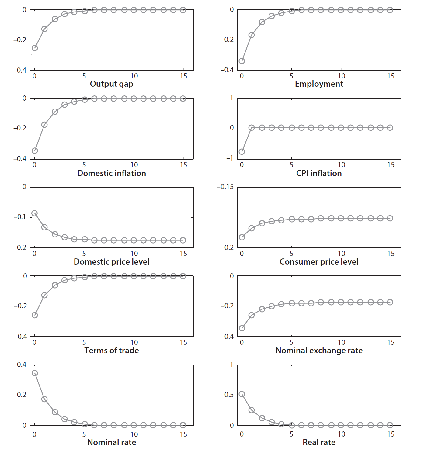
Monetary Policy in the Open Economy

In the beginning of the course, we will extend the New Keynesian (NK) model to the open economy. Why is the NK extension to the open economy so important? Mainly because many policy relevant questions involve open markets:

• What inflation measure should the central bank (CB) stabilize? In an open economy, there are multiple measures of inflation: domestic inflation or CPI, which includes imported goods. Normally, CPI is the relevant measure for economic fluctuations.
• Should the CB care about the exchange rate?
• Is cooperation among CBs desirable? In open economies, outcomes are affected by multiple policymakers. Chances are that cooperation leads to welfare gains.
• How should monetary policy be conducted in a currency union? That is, without collapsing it to the closed economy scenario? Different members may be subject to idiosyncratic shocks, making the answer not trivial..

Modeling open economies requires several decisions about the assumptions that characterize the models. These include several properties listed below. To begin with, the size of the economy (relative to the resto of the world, RoW), since the RoW matters for feedback effects between domestic and foreign quantities. Naturally, small open economies are easier to treat as they assume no feedback effects. The small open economy assumption fails in two-countries models. In a closed economy, we assumed a representative consumer. In that case, the completeness of financial markets and the nature of the available assets was irrelevant: in equilibrium, no trade in assets occurs. Things are different in open economies: at the very least, there are consumers belonging to different economies - a source of heterogeneity -, that can trade in assets. Then, the specific assets that can be traded will matter for equilibrium allocations. In the context of monetary models, the currency in which prices are set matters and has important implications. It is also not obvious what is the right decision on the matter of pricing. A firm producing a goods in our economy might decide to set the price of the exported good in terms of the domestic, foreign, or a third-party currency. These cases have different implications and are relevant in different contexts to model different phenomena. Last, models of open economies can be interpreted as a particular case of heterogeneous agent models, where heterogeneity arises by the country of belonging. Idiosyncratic shocks and country-specific constraints incorporate such heterogeneity.

The following framework is derived from Chapter 8 of the textbook, which is itself a slightly simplified version of Galí and Monacelli (2005). Its assumptions are strong, but characterize an idealized monetary small open economy that serves as a benchmark for relaxing the assumptions. In particular, we assume an infinitesimally small economy with complete markets and producer currency pricing (PCP) (then, the RoW is treated as a closed economy). A representative household maximizes:

$${\mathbb{E}}_0\sum _{t=0}^{\infty }{\beta }^{t}U(C_t,N_t;Z_t)$$

where the consumption bundle has two layers, a CES function of two indices (domestic products $H$ and foreign $F$)

$$C_t\equiv {\left((1-v{)}^{\frac{1}{\eta }}{C}_{H,t}^{\frac{\eta -1}{\eta }}+v{C}_{F,t}^{\frac{\eta -1}{\eta }}\right)}^{\frac{\eta }{\eta -1}}$$

Note that $v$ determines the weight of foreign goods in the consumption bundle, while $\eta$ measures the elasticity of substitution between domestic and foreign goods, so that $1-v$ can be interpreted as a measure of the “home bias”¹. In equilibrium, this is the ratio of domestic goods against foreign goods. The period budget constraint is:

$${\int }_0^1{P}_{H,t}(i)C_{H,t}(i)di+P_{F,t}{C}_{F,t}+{\mathbb{E}}_t[Q_{t,t+1},D_{t+1}]\le W_t{N}_t+D_t$$

where, since we assumed complete markets, we define $D_{t+1}$ as the random payoff next period, while $Q_{t,t+1}$ is the stochastic discount factor (SDF).

Complete Markets, Time- $t$ Trade

This callout summarizes ideas developed more deeply in AMIII (Priit Jeenas). The market value at time $t$ of random payoff $D_{{}_{T+1}}$ is:

$$\begin{array}{rl}\sum _{{\omega }^{t+1}\mid {\omega }^t}V({\omega }^t;{\omega }^{t+1})D({\omega }^{t+1})& =\sum _{{\omega }^{t+1}\mid {\omega }^t}\xi ({\omega }^{t+1}\mid {\omega }^t)\frac{V({\omega }^t);{\omega }^{t+1}}{\xi ({\omega }^{t+1};{\omega }^t)}D({\omega }^{t+1})\\ & ={\mathbb{E}}_t[Q_{t,t+1}{D}_{t+1}]\end{array}$$

where $\xi$ is a probability measure.

For simplicity, we assume the same CRRA utility function as in the closed economy:

$$U(C_t,N_t;Z_t)=\{\begin{array}{ll}\left(\frac{C_t^{1-\sigma }-1}{1-\sigma }-\frac{N_t^{1+\varphi }}{1+\varphi }\right)Z_t& \sigma \ne 1\\ \left(\log (C_t)-\frac{N_t^{1+\varphi }}{1+\varphi }\right)Z_t& \sigma =1\end{array}$$

The optimal allocation of expenditure follows as usual, although it now involves two nested levels: the optimal bundle of domestic goods $i$, and the optimal composition of domestic to foreign bundles. For domestic goods, it holds that:

$$C_{H,t}(i)={\left(\frac{P_{H,t}(i)}{P_{H,t}}\right)}^{-\epsilon }{C}_{H,t}$$

for the price level index defined as usual as $P_{H,t}\equiv {\left({\int }_0^1{P}_{H,t}(i{)}^{1-\epsilon }di\right)}^{\frac{1}{1-\epsilon }}$, and now referred to as the domestic price index (DPI). As usual, this implies that ${\int }_0^1{P}_{H,t}(i)C_{H,t}(i)di=P_{H,t}{C}_{H,t}$. As for the domestic against foreign level, this is solved taking the minimization problem:

$$\underset{C_{H,t},C_{F,t}}{\min }{P}_{H,t}{C}_{H,t}+P_{F,t}{C}_{F,t}\text{ subject to }[(1-v{)}^{\frac{1}{\eta }}{C}_{H,t}^{\frac{\eta -1}{\eta }}+v^{\frac{1}{\eta }}{C}_{F,t}^{\frac{1-\eta }{\eta }}{]}^{\frac{1}{\eta -1}}=C_t$$

Then:

$$\begin{array}{rlrl}{C}_{H,t}& =(1-v){\left(\frac{P_{H,t}}{P_t}\right)}^{-\eta }& C_{F,t}& =v{\left(\frac{P_{F,t}}{P_t}\right)}^{-\eta }\end{array}$$

where $P_t\equiv [(1-v)P_{H,t}^{1-\eta }+v{P}_{F,t}^{1-\eta }{]}^{\frac{1}{1-\eta }}$ is referred to as the consumer price index (CPI). As before, this can be rewritten as:

$$P_t{C}_t=P_{H,t}{C}_{H,t}+P_{F,t}{C}_{F,t}$$

The rest of the optimality conditions do not involve foreign variables, and follow similarly as the closed economy case. First, consider the intratemporal optimality condition or optimal labor supply:

$$\frac{W_t}{P_t}=C_t^{\sigma }{N}_t^{\varphi }$$

Then, note the shape of Arrow security optimality condition. Although implicit in the closed economy, we can write it fully:

$$\frac{U_c({\omega }^t)}{P({\omega }^t)}V({\omega }^t;{\omega }^{t+1})=\xi ({\omega }^{t+1}\mid {\omega }^t)\frac{\beta U_c({\omega }^{t+1})}{P({\omega }^{t+1})}$$

Put simply, it imposes that today’s welfare loss associated with the purchase of a specific Arrow security must be equal to the expected gain in utility in the foreign period associated with such security. Exploiting the definition of the SDF, this condition implies the good old condition:

$$Q_{t,t+1}=\beta {\left(\frac{C_{t+1}}{C_t}\right)}^{-\sigma }\left(\frac{Z_{t+1}}{Z_t}\right)\left(\frac{P_t}{P_{t+1}}\right)$$

In this formulation, it is clear that we can isolate the one-period nominally riskless bond. This synthetic asset is crucial, as we will treat the interest rate as the inverse of its price (by definition).

$$\begin{array}{rl}{Q}_t& \equiv e^{-i_t}\\ & ={\mathbb{E}}_t[Q_{t,t+1}]\\ & =\beta {\mathbb{E}}_t\left[{\left(\frac{C_{t+1}}{C_t}\right)}^{-\sigma }\left(\frac{Z_{t+1}}{Z_t}\right)\left(\frac{P_t}{P_{t+1}}\right)\right]\end{array}$$

which can be loglinearized into the consumption analogue of the IS equation:

$$c_t={\mathbb{E}}_t[c_{t+1}]-\frac{1}{\sigma }(i_t-{\mathbb{E}}_t[{\pi }_{t+1}]-\rho )+\frac{1}{\sigma }(1-{\rho }_z)z_t$$

Uncovered Interest Parity Condition

To begin with, state the pricing equation for foreign short-term bond as implied by the uncovered interest parity condition (UIP): $Q_t^{\ast }\equiv e^{-i_t}={\mathbb{E}}_t\left[Q_{t,t+1}\left(\frac{{\mathcal{E}}_{t+1}}{{\mathcal{E}}_t}\right)\right]$.

This can be seen as follows. The price of a foreign bond from a domestic perspective is ${\mathcal{E}}_t{Q}_t^{\ast }$ where the former is the nominal exchange rate (conventionally defined as the ration of foreign to domestic currency), while the latter is the price of the foreign short term riskless bond. It must be the case that ${\mathcal{E}}_t{Q}_t^{\ast }={\mathbb{E}}_t[Q_{t,t+1}{\mathcal{E}}_{t+1}]$, which can be rearranged in the previous expression. Rewrite this as:

$$\begin{array}{rlrl}1& ={\mathbb{E}}_t[e^{i_t}{Q}_{t,t+1}]& 1& ={\mathbb{E}}_t[e^{i_t^{\ast }}\frac{{\mathcal{E}}_{t+1}}{{\mathcal{E}}_t}{Q}_{t,t+1}]\end{array}$$

Subtracting one from the other, and writing the RHS as the exponential function of the logs, it is possible to take the log and then approximate to a first order expansion, so as to respectively obtain:

$$\begin{array}{rl}0& ={\mathbb{E}}_t[Q_{t,t+1}(e^{i_t}-e^{i_t^{\ast }+\Delta {ϵ}_{t+1}})]\\ i_t& \approx i_t^{\ast }+{\mathbb{E}}_t[\Delta {ϵ}_{t+1}]\end{array}$$

Obviously, the second is a linear approximation: it kills the “risk premium” that is naturally incorporated in the UIP condition in the form of the “spread”.

To continue, define the terms of trade as: ${\mathcal{S}}_t\equiv \frac{P_{F,t}}{P_{H,t}}$. In logs:

$$s_t=p_{F,t}-p_{H,t}$$

The CPI and domestic price indices are defined as before. The terms of trade involve nominal variable; as in the closed economy case of the domestic price level, it is not possible to Taylor-expand around some “steady state”, as this concept is not well-defined for nominal variables. Then, we rather divide both sides by $P_t$:

$$1=(1-v){\left(\frac{P_{H,t}}{P_t}\right)}^{1-\eta }+v{\left(\frac{P_{F;t}}{P_t}\right)}^{1-\eta }$$

The domestic and foreign prices relative to the CPI, instead, do have a well defined steady state (in particular, in equilibrium, each of them equals one). Rewrite the previous condition in logs:

$$\begin{array}{rl}1& =(1-v){\left(\frac{P_{H,t}}{P_t}\right)}^{1-\eta }+v{\left(\frac{P_{F;t}}{P_t}\right)}^{1-\eta }\\ 1& =(1-v)e^{(1-\eta )(p_{H,t}-p_t)}+v{e}^{(1-\eta )(p_{F,t}-p_t)}\\ 1& \simeq (1-v)(1+(1-\eta )(p_{H,t}-p_t))+v(1+(1-\eta )(p_{F,t}-p_t))\\ 1& \simeq 1+(1-v)(1-\eta )(p_{H,t}-p_t))+v(1-\eta )(p_{F,t}-p_t))\\ 0& \simeq (1-v)(1-\eta )p_{H,t}+v(1-\eta )p_{F,t}-(1-v+v)(1-\eta )p_t\\ 0& \simeq (1-v)p_{H,t}+v{p}_{F,t}-p_t\end{array}$$

This implies the following results:

$$\begin{array}{rl}{p}_t& \simeq (1-v)p_{H,t}+v{p}_{F,t}\\ & =p_{H,t}+v{s}_t\\ {\pi }_t& \simeq {\pi }_{H,t}+v\Delta s_t\end{array}$$

a result that holds exactly rather than approximately for $\eta =1$ since $P_t\equiv P_{H,t}^{1-v}{P}_{F,t}^v$.

Another heroic assumption we impose is that the law of one price (full pass through) holds². That it:

$$\begin{array}{rl}{P}_{F,t}& ={\mathcal{E}}_t{P}_{F,t}^{\ast }={\mathcal{E}}_t{P}_t^{\ast }\\ P_{H,t}^{\ast }& =\frac{P_{H,t}}{{\mathcal{E}}_t}\\ & \\ p_{F,t}& =e_t+p_t^{\ast }\\ p_{H,t}^{\ast }& =p_{H,t}-e_t\end{array}$$

Note that we are treating the rest of the world as a closed economy, since $P_{F,t}^{\ast }=P_t^{\ast }$ is assumed in line 1.

Define the real exchange rate:

$$\begin{array}{rl}{\mathcal{Q}}_t& \equiv \frac{{\mathcal{E}}_t{P}_t^{\ast }}{P_t}=\frac{P_{F,t}}{P_t}\\ q_t& \equiv p_{F,t}-p_t\\ & \simeq p_{F,t}-(p_{H,t}+v{s}_t)\\ & =(1-v)s_t\end{array}$$

also holding exactly for $\eta =1$ and hence $\mathcal{Q}=S_t^{1-v}$.

A very important implication of complete markets is the international risk sharing condition. Foreign consumers also have access to complete markets, and thus face the following optimality condition:

$$\begin{array}{rl}\frac{V({\omega }^t;{\omega }^{t+1})}{P^{\ast }({\omega }^t)\mathcal{E}({\omega }^t)}{U}_c^{\ast }({\omega }^t)& =\xi ({\omega }^{t+1}\mid {\omega }^t)\frac{\beta U_c^{\ast }({\omega }^{t+1})}{P_{{\omega }^{t+1}}^{\ast }\mathcal{E}({\omega }^{t+1})}\\ ⟹\frac{U_{c,t}^{\ast }}{{\mathcal{Q}}_t{U}_{c,t}}& =\frac{U_{c,t+1}^{\ast }}{{\mathcal{Q}}_{t+1}{U}_{c,t+1}}\end{array}$$

where the second line is obtained dividing the asset optimality conditions for home and foreign. That constant ratio can be referred to as $\frac{U_{c,t}^{\ast }}{{\mathcal{Q}}_t{U}_{c,t}}=\vartheta$. This allows some smart rewriting:

$$\begin{array}{rl}{C}_t& =\vartheta C_t^{\ast }{Z}_t^{\frac{1}{\sigma }}{\mathcal{Q}}_t^{\frac{1}{\sigma }}\\ c_t& =y_t^{\ast }+\frac{1}{\sigma }(z_t+q_t)\\ & \simeq y_t^{\ast }+\frac{1}{\sigma }{z}_t+\left(\frac{1-v}{\sigma }\right)s_t\end{array}$$

which implies in equilibrium a perfect co-movement between domestic consumption and foreign output (hence the name). Note that this condition is normally rejected empirically (Backus-Smith puzzle).

To continue, define an export function that will be part of the aggregate demand for domestic goods. Anything can be assumed in this case, thanks to the assumption that home is infinitesimally small. By analogy with the demand function, impose that:

$$X_t(i)={\left(\frac{P_{H,t}(i)}{P_{H,t}}\right)}^{-\epsilon }{X}_t$$

where $X_t\equiv {\left({\int }_0^1{X}_t(i{)}^{\frac{\epsilon -1}{\epsilon }}di\right)}^{\frac{\epsilon }{\epsilon -1}}$ is given by:

$$\begin{array}{rl}{X}_t& =v{\left(\frac{P_{H,t}}{{\mathcal{E}}_t{P}_t^{\ast }}\right)}^{-\eta }{Y}_t^{\ast }\\ & =v{\mathcal{S}}_t^{\eta }{Y}_t^{\ast }\end{array}$$

With a symmetric steady state, balanced trade follows: $C_F=X_t$. This setup is consistent with a global GE with a continuum of countries (for reference, read Galí and Monacelli’s response to Hellwig).

Optimal price setting remains the same as usual, as it does not involve any open economy term. This holds, of course, only given that the firms sets a unique price by the full pass through assumption. For details about this derivation, refer to the previous LNs.

The domestic inflation dynamics follow as:

$${\pi }_{H,t}=\beta {\mathbb{E}}_t[{\pi }_{H,t+1}]-\lambda ({\mu }_t-\mu )$$

Note that his involves domestic inflation, and will not hold for CPI. The key message is that the markup based version of the NKPC for domestic inflation is invariant to openness.

To solve for the equilibrium, impose market clearing on the final goods markets:

$$\begin{array}{rl}{Y}_t(i)& =C_{H,t}(i)+X_t(i)\\ & ={\left(\frac{P_{H,t}(i)}{P_{H,t}}\right)}^{-\epsilon }{C}_{H,t}+{\left(\frac{P_{H,t}(i)}{P_{H,t}}\right)}^{-\epsilon }{X}_t\\ & ={\left(\frac{P_{H,t}(i)}{P_{H,t}}\right)}^{-\epsilon }\left[(1-v){\left(\frac{P_{H,t}(i)}{P_t}\right)}^{-\epsilon }{C}_t+v{S}_t^{\eta }{Y}_t^{\ast }\right]\\ & ={\left(\frac{P_{H,t}(i)}{P_{H,t}}\right)}^{-\epsilon }\left[(1-v)[(1-v)+v{\mathcal{S}}_t^{1-\eta }{]}^{\frac{\eta }{\eta -1}}{C}_t+v{S}_t^{\eta }{Y}_t^{\ast }\right]\end{array}$$

Combined with the definition of output as $Y_t\equiv {\left({\int }_0^1{Y}_t(i{)}^{\frac{\epsilon -1}{\epsilon }}di\right)}^{\frac{\epsilon -1}{\epsilon }}$:

$$Y_t=(1-v){\left[(1-v)+v{\mathcal{S}}_t^{1-\eta }\right]}^{\frac{\eta }{\eta -1}}{C}_t+v{S}_t^{\eta }{Y}_t^{\ast }$$

In the steady state, $C=Y=Y^{\ast }$ and $\mathcal{S}=1$. Log-linearizing around a symmetric steady state, we get that:

$${\hat{y}}_t\simeq (1-v){\hat{c}}_t+v(2-v)\eta s_t+v{\hat{y}}_t^{\ast }$$

with the particular exact result, for $\eta =1$:

$$Y_t=(1-v){\mathcal{S}}_t^v{C}_t+v{\mathcal{S}}_t{Y}_t^{\ast }$$

UIP and the Terms of Trade

Under the assumption of complete international financial markets, the UIP can be log-linearized about a perfect foresight steady state, leading to the familiar UIP reported before. Furthermore, however, we can combine ^3e7256 and the UIP condition to obtain:

$$\begin{array}{rl}{e}_t& ={\mathbb{E}}_t[e_{t+1}]+i_t^{\ast }-i_t\\ \underset{s_t}{\underbrace{e_t+p_t^{\ast }-p_{H,t}}}& ={\mathbb{E}}_t[e_{t+1}+p_{t+1}^{\ast }-p_{H,t+1}]+r_t^{\ast }-r_t\\ s_t& ={\mathbb{E}}_t[s_{t+1}]+r_t^{\ast }-r_t\\ s_t& =\sum _{k=0}^{\infty }{\mathbb{E}}_t[r_{t+k}^{\ast }-r_{t+k}]\end{array}$$

or equivalently:

$$s_t=\sum _{k=0}^{\infty }{\mathbb{E}}_t[(i_{t+k}^{\ast }-{\pi }_{t+k+1}^{\ast })-(i_{t+k}-{\pi }_{t+k+1})]$$

That is, the terms of trade are a function of current and anticipated real interest rate differentials.

Labor market clearing works as in the closed economy scenario:

$$\begin{array}{rl}{N}_t& \equiv {\int }_0^1{N}_t(i)di\\ & ={\left(\frac{Y_t}{A_t}\right)}^{\frac{1}{1-\alpha }}{\int }_0^1{\left(\frac{P_{H,t}(i)}{P_{H,t}}\right)}^{-\frac{\epsilon }{1-\alpha }}di\end{array}$$

approximated as:

$$(1-\alpha )n_t=y_t-a_t$$

The price markup expressed in terms of the output gap is also similar to the basic model, with the addition of the terms of trade:

$${\mu }_t\simeq -\sigma c_t-\left(\frac{\varphi +\alpha }{1-\alpha }\right)y_t-v{s}_t+\left(1+\frac{\varphi +\alpha }{1-\alpha }\right)a_t+\log (1-\alpha )$$

The equilibrium of the non-policy block can be summarized as follows:

$$\begin{array}{rl}{\hat{y}}_t& \simeq (1-v){\hat{c}}_t+v(2-v)\eta s_t+v{\hat{y}}_t^{\ast }\\ {\hat{c}}_t& ={\mathbb{E}}_t[{\hat{c}}_{t+1}]-\frac{1}{\sigma }({\hat{i}}_t-{\mathbb{E}}_t[{\pi }_{t+1}])+\frac{1}{\sigma }(1-{\rho }_z)z_t\\ {\hat{c}}_t& \simeq \left(\frac{1-v}{\sigma }\right)s_t+{\hat{y}}_t^{\ast }+\frac{1}{\sigma }{z}_t\\ {\pi }_{H,t}& =\beta {\mathbb{E}}_t[{\pi }_{H,t+1}]-\lambda {\hat{\mu }}_t\\ \hat{\mu }& =-\sigma c_t-\left(\frac{\varphi +\alpha }{1-\alpha }\right)y_t-v{s}_t+\left(1+\frac{\varphi +\alpha }{1-\alpha }\right)a_t+\log (1-\alpha )\\ {\pi }_t& ={\pi }_{H,t+1}+v\Delta s_t\\ s_t& =s_{t-1}+\Delta e_t+{\pi }_t^{\ast }-p_{H,t}\end{array}$$

for some arbitrary non-policy block. An example might be:

$$i_t=\rho +{\varphi }_{\pi }{\pi }_{H,t}+{\varphi }_y{\hat{y}}_t+v_t$$

---

Footnotes

1. Since we’re infinitesimally small, without home bias no one would buy domestic goods. Weight to such goods needs to be imposed ad hoc. ↩

2. This is often contradicted in practice, by local currency pricing or customer market pricing, even with PCP. ↩