Topics in Macroeconomics II. Expectations and Optimal Policy (Marcet)

Preface by Lorenzo Bianchi Chignoli

These lecture notes were originally prepared for the Topics in Macroeconomics II. Expectation and Optimal Policy course offered by Albert Marcet in the MRes in Economics program at Universitat Pompeu Fabra during the Fall 2025 term. The content is primarily derived from my personal notes. Many of the mathematical derivations were worked out as exercises and, therefore, may contain inaccuracies.

This course explores modelling approaches to expectations, and the corresponding optimal policies in dynamic economies. The two main sections of the notes reflect this structure.

Expectations

History of Rational Expectations

Older approaches simply specified expectations as a fixed functions of current and previous variables, rather than forward looking expectations based on the model’s own laws. Assuming inconsistent expectations to the model’s implication is the most disappointing feature of the non-rational expectations paradigm. The crisis of Classical Keynesian models occurred in the 70s with the failure of the classical Phillips Curve to predict a positive correlation between inflation and unemployment. With rational expectations (hereafter, RE), instead, agent’s predictions coincide with the objective model’s predictions. This also implies that expectations are enforced by the model itself: there is no additional degrees of freedom to test the model predictions against specifications of expectations. Sure enough, the Classical Keynesian models had an excessive, basically infinite amount of degrees of freedom, with maximized explanatory power and minimized predictive power. At that time, RE was a welcome methodological innovation, as it avoided arbitrary model specifications.

Agents in the Old Keynesian models were assumed to form expectations following equations that differed from the model’s equation determining the very outcome expected upon. Put simply, Old Keynesian agents make the same mistake all the time. In contrast, real-world agents do make mistakes, but these are not identical at all times, and do not incur systematic welfare losses due to misspecified expectations. Put simply, Classical Keynesian models were lacking a learning mechanism for people to adjust their expectational equations.

RE, instead, avoided that “stupid” mistakes were repeatedly committed, and became the dominant paradigm in modelling expectations in economics around the 80s. This is thanks to some theoretical features of RE:

• The choice of expectations is dictated by the model, and no arbitrary modelling is admitted.
• It a stable expectation that is maintained in the long run
• It prevents agents to make systematic, or even “stupid”, mistakes in their forecasts. Although these are good methodological justification, and any deviation from RE should address them, it seems like an unreasonable burden that agents come to know rational expectations straight away. Moreover, alternative way to solve such problems may exist.

An Application: Expectations and Asset Prices

An excellent example for modeling expectation is the stock market. Stock prices are quite unpredictable, especially in the long run, where booms and busts dominate the pricing dynamics. The stock market may exhibit high prices either due to good fundamentals, and the corresponding well-grounded expectations of profitability; or mistaken expectations, which may lead to a bubble burst. The conflict between expectations and outcomes is well exemplified by the famed excess return regressions. Fama’s efficient market’s hypothesis should prevent agents from predicting stock prices (read as: to find a large and statistically significant value for a coefficient in the regression of stock prices).

The Efficient Market Hypothesis

The primary role of the capital market is allocation of ownership of the economy’s capital stock. In general terms, the ideal is a market in which prices provide accurate signals for resource allocation: that is, a market in which firms can make production-investment decisions, and investors can choose among securities that represent ownership of firms’ activities under the assumption that security prices at any time ‘fully reflect’ all available information. A market in which prices always ‘fully reflect’ available information is called ‘efficient’. (Fama, 1970, p. 383)

Instead, excess return regressions show this is not quite the case. Consider Table 1 in Adam, Marcet, Nicolini:

Quantity	Coefficient	Other measure
Volatility of PD ratio	${\hat{\mathbb{E}}}_{\mathrm{PD}}=123.91$	${\hat{\sigma }}_{\mathrm{PD}}=62.43$
Persistence of PD ratio	${\hat{\rho }}_{{\mathrm{PD}}_t,{\mathrm{PD}}_{t-1}}=.97$
Excessive return volatility	${\hat{\rho }}_{{\text{R}}_t^{\mathrm{stock}}}=11.44$	${\hat{\sigma }}_{\frac{D_t}{D_{t-1}}}=2.88$
Excess long run return predictability ($n=5$ years)	${\hat{b}}^{\mathrm{PD}}=-.0041$	$R^2=.2102$
Equity premium	${\hat{E}}_{R_t^{\mathrm{stock}}}=2.25$	${\hat{E}}_{R_t^{\mathrm{bond}}}=.15$

where $D_t$ denotes dividends, $P_t$ stock prices, $P{D}_t$ is the price-dividend ratio, and $R$ are the returns for stocks and bonds. This shows that stock prices are highly volatile: not only the standard deviation of the price-to-dividend ratio is extremely high relative to its mean, but also the standard deviation in stock returns are much larger than the standard deviation in dividends. Moreover, fluctuations in PD are persistent. Put simply: If markets are efficient, stock prices ($P_t$) should only move when there is news about the future cash flows (dividends, $D_t$). Therefore, the price-dividend ratio ($P/D$) should be relatively stable unless expected future dividend growth changes, and returns should be unpredictable. Instead, the data shows the $P/D$ ratio is incredibly volatile (${\hat{\sigma }}_{PD}$ is high) and persistent (it stays high or low for a long time). Moreover, prices move around much more than dividends do.

This leads to the famed long run return predictability, incorporated in the excess return regressions (Fama and French, 1992). The test (which is reported in Cochrane’s version) works as follows: When the $D/P$ ratio moves, what happens next? Does it predict that dividends will change? Or does it predict that prices will snap back (mean reversion)? The regressions show that today’s $D/P$ ratio does not predict future dividends (which would be the “efficient” explanation); instead, it predicts future returns. Then, high volatility in prices is not driven by fundamentals (dividends), but rather by fluctuations in expected returns. Prices swing away from fundamentals and then slowly revert back, creating predictable excess returns. Formally, define the total future $n$-period excess returns as

$$X_{t,n}=\sum _{i=1}^n[\log (1+R_{\mathrm{stock},t+i})-\log (1+R_{\mathrm{bond},t+i})]$$

and run the following regressions:

$$\begin{array}{rl}{X}_{t,n}& =a_n+b_n\frac{D_t}{P_t}+u_{t,n}\\ \frac{D_{t+n}}{D_t}& =c_n+d_n\frac{D_t}{P_t}+v_{t,n}\end{array}$$

Empirical results for this regression are provided by Cochrane (2005) as follows:

	Predict $X_{t,n}$			Predict $\frac{D_{t+n}}{D_t}$
$n$	${\hat{b}}_n$	$\sigma ({\hat{b}}_n)$	$R^2$	${\hat{d}}_n$	$\sigma ({\hat{d}}_n)$	$R^2$
1	5.30	2.00	0.15	2.00	1.10	0.06
2	10	3.10	0.23	2.50	2.1	0.06
3	15	4.00	0.37	2.4	2.1	0.06
5	33	5.80	0.6	4.7	2.4	0.12

(Beware that this data has DP rather than PD on the RHS, and data is yearly rather than quarterly like in the previous table.) Put simply, future excess returns are higher when $P$ is low (relative to the dividend it yields). Moreover, $\hat{b}$ is significantly different from 0, the more the longer the horizon $n$. Finally, the $R^2$ is relatively high and rejects the “weak form of market efficiency” in the long run. This result is very robust and is sometimes described as mean reversion of DP. In contrast, $\hat{d}$ is not significant: therefore, mean reversion and volatility of returns are due to price movements, and not dividends.

Let us attempt to micro-found asset pricing with RE. In the famed model by Lucas and Stokey, a representative consumer/investor chooses stock holdings $S_t$ and consumption $C_t$ to solve:

$$\underset{\{S_t,C_t{\}}_{t=0}^{\infty }}{\max }{\mathbb{E}}_0\sum _{t=0}^{\infty }{\beta }^{t}u(C_t)\text{ such that }{C}_t+S_t{P}_t=W_t+S_{t-1}(P_t+D_t)$$

with exogenous $\{W_t,D_t\}$. The stock market is competitive, with a total (normalized) supply of 1. Feasibility is ensured at $C_t=W_t+D_t$ and the stock market equilibrium implies $S_t=1$ (the RA demand equals supply). The FOC for the optimal $S$ is:

$$u^{\prime }(C_t)P_t=\beta {\mathbb{E}}_t[u^{\prime }(C_{t+1})(P_{t+1}+D_{t+1})]$$

which can be plugged into the equilibrium conditions. By forward iteration and LIE (after assuming bounded prices):

$$P_t={\mathbb{E}}_t\sum _{j=1}^{\infty }{\beta }^j\frac{u^{\prime }(C_{t+j})}{u^{\prime }(C_t)}{D}_{t+j}$$

Given that consumption is fixed by the feasibility condition, in equilibrium this expectation is a function of past $(W,D)$‘s only. Notice that in principle the $C_t$ that solves investors’ problem should be a function of past stock demand; however, stock holdings are not a state variable on equilibrium. More formally, for a history profile $(W,D{)}^t\equiv (W_t,D_t,W_{t-1},D_{t-1},\dots ,W_0,D_0)$, it holds that prices should be predicted as a function of exogenous processes up to history time $t$, with no role of prices in predictions:

$$P_t=F_t^P(\{W_i,D_i{\}}_{i=0}^t)$$

for some non-stochastic pricing function $F_t^P$.

However, Cochrane’s (2005) regressions show that it is virtually possible to “predict the future”: high prices systematically accompany price drops (recall, the ratio is dividend-to-prices in Cochrane’s regressions). Positive, but not significant, results are also obtained for dividends predictions. Thus, something is much strongly incorporated in prices that in cash flows — that is, actual profitability. Something else might affect this difference, as the fundamental does not seem to suffice. Moreover, the model assumes that agents actually know the non-stochastic pricing function since their birth. The only uncertainty lies in the stochastic process for the exogenous variables.

Assuming RE leads to serious puzzles once we get to the data. For instance, the equity premium puzzle (Mehra and Prescott, 1982), and especially Shiller’s (1981) excess volatility puzzle. Both phenomena are difficult to explain through rational expectations. Intuitively, the reasons is that under RE it is in general difficult to explain stock prices volatility in the equation

$$P_t={\mathbb{E}}_t\sum _{j=1}^{\infty }{\beta }^j\frac{U^{\prime }(C_{t+j})}{U^{\prime }(C_t)}{D}_{t+j}$$

In fact, averaging dividends (twice: the expectation is a probabilistic average, over a time series which also serves as an average) implies that volatility should drop dramatically. If this equation would hold, then, it would be unlikely that prices are more volatile than dividends. For precision, consider the risk neutral case $U(C)=C$ to give a structural form to marginal utilities, with no labor income. Assume that dividends follow a pure unit root process such as $\frac{D_t}{D_{t-1}}=a{ϵ}_t$ with $\stackrel{i.i.d.}{\sim }$ error with mean 1. Prices are a discounted sum of the future stream of dividends:

$$P_t={\mathbb{E}}_t\sum _{j=1}^{\infty }{\beta }^j{D}_{t+j}$$

Substituting (and ignoring variance terms in a loglinear approximation):

$$P_t\approx \sum _{j=1}^{\infty }(\beta \alpha {)}^j{D}_t=\frac{\beta a}{1-\beta a}{D}_t$$

which implies that the $PD$ ratio is constant. This contradicts data dramatically, where the $PD$ ratio is highly volatile.

In the subsequent twenty years, many authors actually provided success stories in their attempt to generalize Lucas’ asset pricing model, for instance with more general utility functions, production functions, incomplete markets, heterogeneous agents, and the like. For years, they failed repeatedly to give a quantitative explanation. Some exceptions include the following cases.

Campbell and Cochrane (1999) focus on habits, and defined the utility function:

$$\begin{array}{rl}{\mathbb{E}}_0& \left[\sum _{t=0}^{\infty }{\beta }^{t}u\left(\frac{C_t}{H_{t-1}}\right)\right]\\ \log H_t& =\rho H_{t-1}+\delta \left(\frac{C_t}{C_{t-1}}\right)\left(\frac{C_t}{C_{t-1}}-\log H_{t-1}\right)\end{array}$$

where the stochastic discount factor depends on $H_t$. Since this is highly volatile, this affects the risk aversion which becomes $\mathbb{E}\left[-C_t\frac{u^{\prime \prime }\left(\frac{C_t}{H_{t-1}}\right)}{u^{\prime }\left(\frac{C_t}{H_{t-1}}\right)}\right]\approx 80$. However, this utility function leads to weird results when plugged into standard DSGE models, such as increased utility for decreasing consumption. Because agents care about the gap (relative status), not the absolute amount, they are mathematically happier being poor in a society where everyone else is destitute (low habit), than being rich in a society where everyone else is slightly richer (high habit)¹. Ljungqvist and Uhlig showed that in these models, a government could theoretically burn 10% of the country’s endowment and make everyone happier by ending the “rat race”.

Bansal and Yaron (2004) assume output growth has a slow-moving component that affects dividends, such as $\log D_t-\log D_{t-1}=a_t+{ϵ}_t$ such that $a_t=a_{t-1}+{\eta }_t$. Importantly, $a_t$ is perfectly observed by investors in period $t$. Since $a_t$ is the denominator and $1-\beta a_t\approx 0$, small changes in $a_t$ lead to large changes in prices. This allows to explain the variance in the data. However, some problems still persist. To match, the data, the variance of $\eta$ should be very small, because dividend growth does not show a strong unit root behavior in practice. If the variance of $\eta$ is much smaller than the variance of ${ϵ}_t$, then this will assume a huge role as it piles up in the long run. The growth rate becomes time-varying and can exhibit large fluctuations; moreover, since the denominator is close to 1, small fluctuations in lead to large fluctuations in the growth rate. Yet, it is weird to assume that agents in the model know about a variable, $a_t$, which does not even exist in statistical agencies.

Last, the rare disasters literature is also an example of success of RE. In this case, ${\mathbb{E}}_t[u^{\prime }(C_{t+1})]$: a small probability multiplies a very large number; then, taking the variance of consumption does not provide good insights on the variance of marginal utility, that could explode due to rare disasters. The main criticism, however, sounds as follows: if the truth is that these “small perceived probabilities” matter so much for asset pricing, then how can we ever know anything about stock price behavior? This is very close to a purely behavioral story where agents’ arbitrary changes in expectations can matter a lot.

Summing up, these attempt are starting to resonate familiar with the late-70s strategy. It is always possible to cook up models where a flawed assumption can explain some phenomena ex post, despite being basically useless for ex ante prediction. Moreover, survey data suggest that even professional forecasters are not following RE that explain the evolution of quantities such as the PD ratio (Adam, Marcet and Beutel, AER 2017). RE is not the only way to attain the objectives desired by Sargent, Prescott, Lucas, and many others. With the additional contribution of the GFC, non-RE are being liberalized in these years, although this still faces a strong resistance. In fact, a mainstream argument is that departures from RE should be temporary — any learning feature should converge rapidly to RE. This is usually referred to as the Friedman hypothesis.

Market Selection Hypothesis or Friedman Hypothesis

Investors that hold wrong beliefs will be driven out of the market very quickly.

However, recent evidence suggests that not only learning, but also expulsion from the market takes a lot of time. Moreover, overly optimistic “crazy” agents may be overly parsimonious, and their savings may still ferry them to the future market (despite present welfare losses).

A formal test of RE through surveys

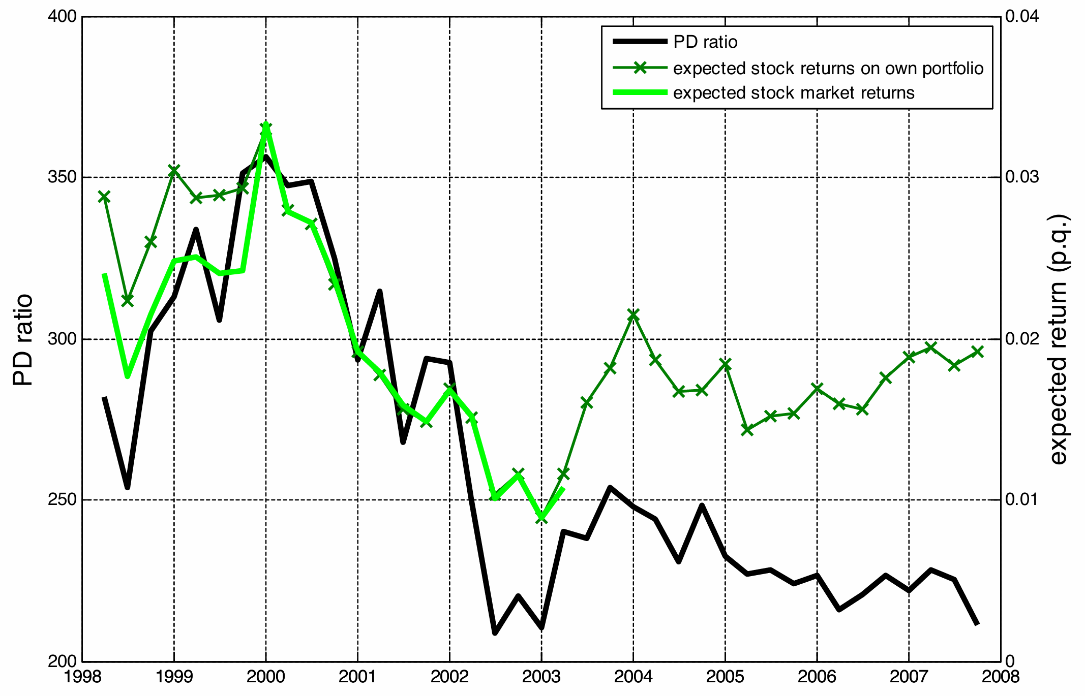
This graphs shows the median stock returns over investors that answers the survey, and should represent the “consensus belief”. Investors were most optimistic about stock returns at the top of the dot.com bubble (December, 1999). However, excess return regressions would have suggested that future returns were on average low at the top of the bubble (that is, high PD). Put simply, the green line in the graph seems incompatible with both RE among investors and data-driven prediction of the excess return regressions. Note that this plot suggest a positive correlation between PD and expected returns:

Survey	Correlation
UBS Gallup 1yr	.79
Shiller Survey 1yr	.38
Shiller Survey 10yr	.66

while their empirical correlation is negative!

It is possible to utilize a formal test for the idea that investors’ expectations do not instance RE nor excess-return ideas (Adam, Marcet and Beutel, 2017). Observed expectations are defined as $S_{t,n}={\mathbb{E}}_t^{\mathcal{P}}[R_{t,n}]+v_t$ where the first term represents expectations and $v_t$ is a measurement error (agents might also report inconsistently, as they might not be sure about their opinions). The test constructs a comparison between expectations and reality. It shows that investors are not rational because they are pro-cyclical (optimistic when prices are high) while the actual market is counter-cyclical (returns are low when prices are high). This is why the notes state that “a good model should match these variables, but this is not the case” for RE models. Define:

• Survey expectations, ${\mathcal{S}}_{t,n}$ This is the subjective expected return coming from surveys (e.g., the UBS/Gallup survey or Shiller’s survey) where they ask investors: “How much do you expect the stock market to return over the next year?“. It should incorporate the relationship: ${\mathcal{S}}_{t,n}\approx {\mathbb{E}}_t^{\mathcal{P}}[R_{t,n}]$.
• Realized returns, $R_{t,n}$. This is the objective actual return that occurred in the market over that same period. ${\mathbb{E}}_t[R_{t,n}]$ is the true mathematical expectation.

Regress:

$${\mathcal{S}}_{t,n}=a^n+{\varphi }^n\frac{P_t}{D_t}+u_t^n$$

to find an estimate ${\hat{\varphi }}^n$. Then, regress:

$$R_{t,n}=a^n+{\bar{\varphi }}^n\frac{P_t}{D_t}+U_t^n$$

to find an estimate ${\hat{\bar{\varphi }}}^n$. Under RE, these should be identical, since the residual should still be orthogonal to the regressions. In fact, plugging in ${\mathcal{S}}_{t,n}={\mathbb{E}}_t[R_{t,n}]+v_t$ for the true expectation $\mathbb{E}$ into ^1177f5:

$$R_{t,n}=a^n+{\varphi }^n\frac{P_t}{D_t}+u_t^n-v_t+{ϵ}_{t+n}^n$$

for the true prediction error ${ϵ}_{t+n}^n$. Clearly, $\mathbb{E}\left[(u_t^n-v_t+{ϵ}_{t+n}^n)\frac{P_t}{D_t}\right]=0$ because $u$ is a regression error, $v$ is a measurement error assumed as orthogonal, and ${ϵ}_{t+n}^n$ is a “true” forecasting error. The hypothesis ${\varphi }^n={\bar{\varphi }}^n$ can be tested by SURE and is, in fact, rejected:

Survey measure	${\hat{\varphi }}^n\cdot 10^3$	${\hat{\bar{\varphi }}}^n\cdot 10^3$	p value
UBS*, all, 1yr, Michigan	0.53	-2.93	0.0000
Shiller, 1yr, Michigan	0.28	-1.48	0.0000
Shiller, 10yr, Michigan	3.51	-6.48	0.0000

This regression also allows to attempt model matching. A good model should match there variables, but this is not the case: they even have opposite signs.

• Reality ($\hat{\bar{\varphi }}<0$): When $P/D$ is high (market is expensive), future returns are low (mean reversion).
• Beliefs ($\hat{\varphi }>0$): When $P/D$ is high (market is expensive), investors expect future returns to be high.

A similar test was developed by Coibion and Gorodnichenko as:

$$R_{t,n}-{\mathcal{S}}_{t,n}=A^n+B^n\frac{P_t}{D_t}+{ϵ}_t$$

or similarly

$$R_{t,n}-{\mathcal{S}}_{t,n}=A^n+B^n(R_{t-n},n-{\mathcal{S}}_{t-n,n})+{ϵ}_t$$

where the null (rejected) is $B^n=0$. The test is identical to AMB, since $B^n=\overline{{\varphi }^n}-{\varphi }^n$.

Asset Prices under Bayesian-RE and Disagreement

Learning about Fundamental shocks

In Bayesian models, agents do not know all the moments of the fundamental data generating process. In this section, we analyze a model of learning about fundamental shocks. This model is interesting to explore if Bayesian RE converge to RE, and if so how fast, and whether Bayesian RE can be used as a bounded substitute for RE.

Consider a special case of Lucas’ model with no risk aversion $u(C)=C$ and $W_t=0$. The growth rate of dividends follows $\frac{D_t}{D_{t-1}}=1+G+{ϵ}_t$ with mean zero $\stackrel{i.i.d.}{\sim }$ error. Under RE, this case implies ${\mathbb{E}}_t{D}_{t+j}=(1+G{)}^j{D}_t$. Therefore, under RE:

$$\begin{array}{rl}{P}_t& =\sum _{j_{=}0}^{\infty }{\beta }^j(1+G{)}^j{D}_t\\ & =\frac{\beta (1+G)}{1-\beta (1+G)}{D}_t\end{array}$$

which implies a constant PD ratio.

Let us now introduce learning about dividends in this special case. Assume agents don’t know the value of $G$, but have an initial belief about the growth rate such as:

$$1+G\sim \mathcal{N}(m_0,{\sigma }_0)$$

Other than this, they know that $D_t$ follows the process described in ^2a7dd9. Agents have a fully consistent model of dividends and they use this to evaluate their utility. The only deviation from Lucas’ model is that investors maximize the expectation given agents’ imperfect knowledge about the dividend process, ${\tilde{\mathbb{E}}}_t$. Thus, agents do not maximize the true distribution, and rather the distribution conditional on their imperfect knowledge about the dividend process. For a $t=0$ perspective, this is equivalent to $\frac{D_t}{D_{t-1}}=\mathcal{N}(m_0,{\sigma }_0+{\sigma }_{ϵ})$. Given the information at $t$, this is equivalent to $\mathcal{N}(m_t,P_t^e)$, where $P_t^e={\text{Var}}_t(a_t)={\mathbb{E}}_t(a_t-\underset{m_t}{\underbrace{{\mathbb{E}}_t[a_t]}}{)}^2$, where $a_t$ denotes the random variable representing the hidden trend in the Kalman filter. Thus, optimal behavior implies:

$$P_t={\tilde{\mathbb{E}}}_t\sum _{j=1}^{\infty }{\beta }^j\frac{u^{\prime }(C_{t+j})}{u^{\prime }(C_t)}{D}_{t+j}$$

To compute this, remember that agents know the likelihood of $D$ but don’t know $G$. Since they know the model:

$$\begin{array}{rl}{\tilde{\mathbb{E}}}_t& ={\tilde{\mathbb{E}}}_t\left[\prod _{i=1}^j(1+G+{ϵ}_{t+j})D_t\right]\end{array}$$

By $\stackrel{i.i.d.}{\sim }$ error with zero mean, ${\tilde{\mathbb{E}}}_t{D}_{t+j}=D_t{\sum }_{j=1}^{\infty }{\beta }^j{\tilde{\mathbb{E}}}_t[(1+G{)}^j]$. Taking an approximation, ${\tilde{\mathbb{E}}}_t[(1+G{)}^j]\approx ({\tilde{\mathbb{E}}}_t[1+G]{)}^j$, so that:

$$P_t\approx \frac{\beta m_t}{1-\beta m_t}{D}_t$$

To find $m_t$ in a general setup, we resort to the Kalman filter. A summary is provided below.

The Kalman Filter

Consider a multivariate system:

$$\begin{array}{rl}{x}_t& =B{a}_t+{ϵ}_t\\ a_t& =C{a}_{t-1}+{\eta }_t\end{array}$$

with $\stackrel{i.i.d.}{\sim }$ zero-mean errors. The perceived distribution for initial $a_0$ (the prior, $f_{a_0}$) is fixed. All parameters $B,C$ and the distributions of the errors are known. While $a$ is the unobserved “true” state, $x$ is the observed signal, which we must forecast based on previous values. Note that $\mathbb{E}[x_{t+1}|x^t]=C\mathbb{E}[a_t|x^t]$ for a history $x^t\equiv (x_t,x_{t-1},\dots ,x_0)$. Therefore, the problem boils down to finding $m_t\equiv \mathbb{E}[a_t|x^t]$. In a general, non-linear setup we should keep track of the entire posterior distribution of $a$, and all previous values in history $x^t$ would be needed to formulate $m_t$. In the Kalman filter, however, the formula for $m_t$ is recursive under the following assumptions:

• Parameters $B,C$ are known, together with the linear law of motion in ^fba960
• $ϵ,\eta$ are Gaussian with known variances
• The initial perceived distribution is also Gaussian: $a_0\sim f_{a_0}=\mathcal{N}(m_0,{\sigma }_0)$ If these hold, then $m_t$ is a function of $m_{t-1}$ and $x_t$.

For the univariate case (in particular, the ^4c17be), the optimal forecasts are given by:

$$m_t=m_{t-1}+\frac{1}{{\alpha }_t}(x_t-m_{t-1})$$

where

$$\begin{array}{rl}{\alpha }_{t+1}& =1+\frac{{\alpha }_t}{1+{\alpha }_t\frac{{\sigma }_{\eta }^2}{{\sigma }_{ϵ}^2}}\\ {\alpha }_1& =\frac{{\sigma }_{\eta }+{\sigma }_{ϵ}+{\sigma }_0}{{\sigma }_{\eta }+{\sigma }_0}\end{array}$$

For illustration, consider these cases:

• Case 1: ${\sigma }_{\eta }=0$ and ${\sigma }_0=\infty$. In this case, $G$ is a constant and we have no prior knowledge, as in classical econometrics. Then, one can work out that the previous formulae yield ${\alpha }_t=t$ and $m_t={\bar{m}}^{t-1}=\frac{1}{t}{\sum }_{i=1}^t{x}_i$, the simple sample average.
• Case 2: ${\sigma }_0\in \mathbb{R}$, as in Bayesian econometrics. Then, $m_t=\frac{1}{t+{\alpha }_1}\left({\sum }_{i=1}^t{x}_i+{\alpha }_1{m}_0\right)$ is the Bayesian posterior mean.
• Case 3: ${\sigma }_{\eta }>0$ and ${\sigma }_0\in \mathbb{R}$, as in time varying VARs. That is, $a$ is an unobserved time-varying ex ante growth rate that follows a unit root process. In this case, it holds that the gain ${\alpha }_t\to {\alpha }^{\mathrm{ss}}$, where the latter solves:

$${\alpha }^{\mathrm{ss}}=1+\frac{{\alpha }^{\mathrm{ss}}}{1+{\alpha }^{\mathrm{ss}}\frac{{\sigma }_{\eta }^2}{{\sigma }_{ϵ}^2}}$$

Most papers take this relationship in the long run and consider ^ccc7ed as:

$$m_t=\frac{1}{\alpha }\sum _{i=1}^t{\left(1-\frac{1}{\alpha }\right)}^i{x}_{t-1}+{\left(1-\frac{1}{\alpha }\right)}^{t+1}{m}_0$$

so that $m$ is a geometric average of its past values. The steady state gain $\frac{1}{\alpha }$ is lower for a higher ${\sigma }_{ϵ}^2$, meaning that if the transitory shock $ϵ$ has higher variance, less weight is put on recent observations.

Disagreement

Once we consider deviations from RE, we open the door to considering different perceptions across investors: disagreement. The paper by Vissing-Jorgensen (2004) reports the standard deviation of expected returns across investors interviewed in the survey. Disagreement is large and, interestingly, larger at the peak of the dot.com bubble. Many papers find similar patterns for other periods and other assets.

Consider a Lucas’ model with two heterogeneous agent RE, where the source of heterogeneity lies in the discount factor, which is individual-specific. Each household maximizes:

$$\begin{array}{c}\underset{\{S_t^i,C_t^i\}}{\max }{\mathbb{E}}_0\sum _{t=0}^{\infty }({\beta }_i{)}^t{u}_i(C_{i,t})\\ \text{ such that }{C}_{i,t}+S_{i,t}+\sum _{\omega }{p}_{t,b}(\omega )b_{i,t}(\omega )=W_{i,t}+S_{i,t-1}(P_t+D_t)+b_{i,t-1}({\omega }_t)\end{array}$$

In a complete market, agents can trade contracts for every possible future state of the world, which allows them to share risk perfectly. When markets are complete, the First Welfare Theorem applies, and the competitive equilibrium is Pareto-efficient. The FOCs are:

$$\begin{array}{rl}{u}_i^{\prime }(C_{i,t})P_t& =\beta {\mathbb{E}}_t[(u^i{)}^{\prime }(C_{t+1}^i)(P_{t+1}+D_{t+1})]\\ P_t& ={\mathbb{E}}_t\sum _{j=1}^{\infty }({\beta }^i{)}^j\frac{(u^i{)}^{\prime }(C_{t+1}^i)}{(u^i{)}^{\prime }(C_t^i)}{D}_{t+j}\end{array}$$

The problem can be solved from the perspective of a planner with Pareto weights $\alpha$ without prices of bonds²:

$$\begin{array}{c}\underset{\{C_t^1,C_t^2\}}{\max }\alpha {\mathbb{E}}_0\left[\sum _{t=0}^{\infty }({\beta }^1{)}^t{u}^1(C_t^1)\right]+(1-\alpha ){\mathbb{E}}_0\left[\sum _{t=0}^{\infty }({\beta }^2{)}^t{u}^2(C_t^2)\right]\\ \text{such that }{C}_t^1+C_t^2=W_t^1+W_t^2+D_t\equiv {\mathbf{W}}_t\end{array}$$

with FOC:

$$\begin{array}{rl}\frac{(u^1{)}^{\prime }(C_t^1)}{(u^2{)}^{\prime }(C_t^2)}& ={\left(\frac{{\beta }^2}{{\beta }^1}\right)}^t\frac{1-\alpha }{\alpha }\end{array}$$

this FOC, combined with the feasibility condition, allows to solve for the $C$s. So, given some $\alpha$, each consumption path is a fixed function of total output ${\mathbf{W}}_t$, and the pricing equation finally yields $P$.

So far, we assumed that agents are homogeneous, apart from the following:

• Different $W^i$ leading to full risk sharing. Moreover, if $u^i$ are CRRA with same RRA coefficient, prices are just the same as if there were a unique representative agent (see ^65722f which implies Gorman aggregation as a specific case).
• Different utility. Suppose $u^1(\cdot )$ is concave, but $u^2(C)=C$. Then, agent 2 perfectly insures agent 1.
• Different discount factors. If ${\beta }^1<{\beta }^2$, then ${\lim }_{n\to \infty }{c}_t^1=0$. However, in all these cases, both agents affect the pricing of the stock.

Things change when agents disagree about how to forecast $D,W$. For simplicity, assume that agents are otherwise homogeneous, and focus on Markov models where the conditional density is $f_{t-1}(D_t,W_t|(D,W{)}^{t-1})=\mu (D_t,W_t;D_{t-1},W_{t-1})$ for a time-invariant function $\mu$. In particular, denote ${\mu }_t\equiv \mu (D_t,W_t;D_{t-1},W_{t-1})$. The density or likelihood of the observed sample is, thus, $f((D,W{)}^t)={\prod }_{j=1}^t{\mu }_j$. Now, assume that investor $i$ knows that $D,W$ is Markov, but they maintain individual forecasting functions for the divided and wage processes, that is $f_t(D_t,W_t|(D,W{)}^{t-1})={\mu }^i(D_t,W_t;D_{t-1},W_{t-1})$. To the extent that $\mu \ne {\mu }^i$, RE are obviously not satisfied. To the extent that ${\mu }^1\ne {\mu }^2$, disagreement takes place. Now, $i$‘s utility is given by ${\tilde{\mathbb{E}}}_0^i{\sum }_{t=0}^{\infty }{\beta }^{t}u(C_t^i)$ where ${\tilde{\mathbb{E}}}_t^i$ is computed with ${\mu }^i$. From a general equilibrium standpoint, the fact that the two agents hold different expectations is just equivalent to a case where agents have different utility. Then, the FPWF and SPWF continue to hold under complete markets. Put simply, disagreement does not break the Arrow-Debreu theorem, since different probabilities attached to future states can be incorporated in the utility function, and the Arrow-Debreu theorem only relies on utility functions, regardless that such utility functions differ. Competitive equilibrium solves:

$$\begin{array}{c}\underset{\{C_t^1,C_t^2\}}{\max }\alpha {\tilde{\mathbb{E}}}_0^1\left[\sum _{t=0}^{\infty }({\beta }^1{)}^t{u}^1(C_t^1)\right]+(1-\alpha )\widetilde{{\mathbb{E}}_0^2}\left[\sum _{t=0}^{\infty }({\beta }^2{)}^t{u}^2(C_t^2)\right]\\ \text{such that }{C}_t^1+C_t^2={\mathbf{W}}_t\end{array}$$

for some Pareto weight $\alpha$. The planner FOC is as follows:

$$\begin{array}{rlrl}[C_t^1]& :& \alpha \stackrel{1}{\mathrm{Pr}}(h^t)u^{\prime }(C_t^1(h^t))& =\lambda \\ [C_t^2]& :& (1-\alpha )\stackrel{2}{\mathrm{Pr}}(h^t)u^{\prime }(C_t^2(h^t))& =\lambda \end{array}$$

and can be combined into a unique condition by equating the $\lambda$:

$$\begin{array}{rl}\frac{(u^1{)}^{\prime }(C_t^1)}{(u^2{)}^{\prime }(C_t^2)}& =\frac{1-\alpha }{\alpha }\frac{{\mathrm{Pr}}^2(h^t)}{{\mathrm{Pr}}^1(h^t)}\\ & =\frac{1-\alpha }{\alpha }\prod _{j=1}^t\frac{{\mu }_j^2}{{\mu }_j^1}\\ & =\frac{{\mu }_t^2}{{\mu }_t^1}\frac{1-\alpha }{\alpha }\prod _{j=1}^{t-1}\frac{{\mu }_j^2}{{\mu }_j^1}\\ \frac{u^{\prime }(C_t^1)}{u^{\prime }(C_t^2)}& =\frac{{\mu }_t^2}{{\mu }_t^1}\frac{u^{\prime }(C_{t-1}^1)}{u^{\prime }(C_{t-1}^2)}\end{array}$$

An important result is that disappearance from the market is very slow, basically contradicting the Friedman hypothesis. Advocates for the Friedman hypothesis normally invoke agents who are completely mistaken, or Aumann’s “common knowledge” assumptions. In the first case, agents who attach subjective probability equal to 0 to some state belonging to the support are very quickly expelled from the market. This is because they bet effectively infinite odds against an event that eventually occurs, leading to immediate bankruptcy. In the second case, which relies on Aumann’s agreement theorem or the Blackwell-Dubins result on the “merging of opinions,” agents share common priors and the information structure is common knowledge. In this framework, disagreements are impossible to sustain: agents either instantly converge to the truth or, recognizing the rationality of others, refuse to engage in speculative trade (Milgrom and Stokey (1982) no trade theorems). Here, market efficiency is an assumption of the setup, not a result of evolutionary selection. However, the Friedman hypothesis is wrong in general. If agents have beliefs that are wrong but “absolutely continuous” with respect to the truth (i.e., they assign positive probability to all possible events), and they do not share common priors, they can survive and influence prices for extremely long periods. Consider the case with a mistaken agent and compute the expectation:

$$\begin{array}{rl}{\tilde{\mathbb{E}}}_t^1\left[\frac{{\mu }_{2,t+1}}{{\mu }_{1,t+1}}\frac{u^{\prime }(C_{1,t})}{u^{\prime }(C_{2,t})}\right]& =\int \frac{{\mu }_{2,t+1}}{{\mu }_{1,t+1}}\frac{u^{\prime }(C_{1,t})}{u^{\prime }(C_{2,t})}{\mu }_{t+1}(\omega )d\omega \\ & =\int {\mu }_{2,t+1}\frac{u^{\prime }(C_{1,t})}{u^{\prime }(C_{2,t})}d\omega \\ & =\frac{u^{\prime }(C_{1,t})}{u^{\prime }(C_{2,t})}\int {\mu }_{2,t+1}d\omega \\ & =\frac{u^{\prime }(C_{1,t})}{u^{\prime }(C_{2,t})}\end{array}$$

Since the ratio satisfies the martingale property (as shown in the derivation), we can take the limit as $t\to \infty$. By the Martingale Convergence Theorem, the random variable must converge to a limit almost surely. If agent 2 is correct (uses the true measure) and agent 1 is “mistaken” (in the sense that their Kullback-Leibler divergence from the truth is positive), then the likelihood ratio of the true agent to the false agent explodes:

$$\underset{t\to \infty }{\lim }\frac{{\mu }_{2,t}}{{\mu }_{1,t}}\to \infty$$

Using the Planner’s FOC, this implies that the ratio of marginal utilities must also explode:

$$\underset{t\to \infty }{\lim }\frac{u^{\prime }(C_{1,t})}{u^{\prime }(C_{2,t})}\to \infty$$

For this ratio to go to infinity, the denominator (agent 1’s marginal utility) stays finite, which forces the numerator (agent 2’s marginal utility) to infinity:

$$u^{\prime }(C_{1,t})\to \infty ⟹C_{1,t}\to 0$$

While the math proves agent 1 eventually consumes 0 (Friedman was right in the infinite long run), the Yan (2008) result shows that the speed of this decay is determined by the Kullback-Leibler divergence between the two beliefs. If agent 1 is “crazy” (beliefs are very different), $\frac{{\mu }_2}{{\mu }_1}$ grows fast and he vanishes quickly. If agent 1 is “smart but slightly wrong” (beliefs are close), $\frac{{\mu }_2}{{\mu }_1}$ grows very slowly and he survives for a long time.

Conclusion: Limits of Market Selection and Aggregation

The Failure of Friedman’s Selection Hypothesis

Put simply, the Friedman hypothesis (that irrational agents go bankrupt and disappear) holds only in very special, extreme cases. For example, if an agent is “dogmatic” and assigns zero probability to an event that actually occurs, they will be blown out of the water by arbitrage (opponents will bet enormously against them). However, in general, as long as agents have absolute continuity (assigning some positive probability to the truth) and avoid risk-neutral behavior, they disappear very slowly and influence prices for decades.

The Failure of Aggregation (“Wealth Distribution” Problem)

Consequently, aggregation does not hold: we cannot use a representative agent shortcut. Because agents differ in their beliefs, they will hold different portfolios. Over time, wealth shifts toward the agent whose beliefs were closer to the realized data. This means that individual consumption depends not just on aggregate endowments ($W_t$), but also on the evolution of subjective probabilities determining who was right in the past. Thus, the likelihood ratio tracking belief accuracy becomes a new, necessary state variable. To compute stock prices, one must now track the entire distribution of wealth between optimistic and pessimistic agents, making the model significantly more complex.

Parameter Uncertainty vs. Model Uncertainty

Finally, there is a subtle philosophical inconsistency in standard Bayesian models. Usually, we assume only expectations on stochastic variables (like dividends) are mistaken. However, agents are assumed to perfectly know the pricing functional $P(\cdot )$: this is equivalent to assuming that they know exactly how the economy works, given the parameters. This implies that behind standard Bayesian learning, there is still a strong RE assumption: agents are assumed to have innate knowledge of the structural equations of the economy. A more realistic approach relaxes this, allowing agents to be mistaken about the pricing function itself, learning the relationship between prices and fundamentals from scratch (Internal Rationality).

Disagreement and Asset Pricing

Asset prices incorporate opinions about stocks. Important results show that, if opinions (in particular, priors) were identical and correct, no trade would occur in equilibrium – the previously mentioned no-trade theorems. A whole body of literature incorporates this idea in the form of “agreeing to disagree”. Important results include that mistaken agents may survive forever (Blume and Easley, 2006) or elicits additional volatility in stock prices. In fact, X-CAPM models show how agents interact in incomplete markets, but does not explain stock market volatility well.

Various papers emphasize that different expectations augment the effects of market frictions. In what follows, we will discuss such effects on debt limits. Suppose there are two possible realizations for aggregate dividends, $s\in \{H,L\}$. The budget constraint for agent $j$ in period $t$ is:

$$c_t^i+\sum _{s\in \{H,L\}}{p}_t^{b,s}{b}_t^i(s)=b_{t-1}^i(s_t)+w_t^i$$

To ensure this maximization problem is well-defined, we must rule out “Ponzi schemes” (where an agent borrows indefinitely without ever repaying). In standard complete market models, this is achieved by the natural Debt limit (or transversality condition), which limits borrowing only to the present value of future income. However, to introduce a market friction, we assume consumers face a tighter, explicit debt limit:

$$b_t^i(s)\ge -B(s)$$

for some finite bound $B(s)>0$. If this imposed limit $B(s)$ is sufficiently large that it never binds, the friction becomes irrelevant, and we recover the standard complete markets allocation (where the agent is only constrained by the true transversality condition). Conversely, if $B(s)$ is tight enough to bind, agents become liquidity constrained, preventing perfect risk sharing.

Consider the case where $B(s)$ binds. The FOCs are, for each agent and bond:

$$\begin{array}{rlrl}{p}_t^{b,s}{u}^{\prime }(c_t^j)& =\delta u^{\prime }(c_{t+1}^j(s_{t+1}=s)){\mu }^{s,j}& \text{ if }{b}_t^j(s)& =-B(s)\\ p_t^{b,s}{u}^{\prime }(c_t^j)& >\delta u^{\prime }(c_{t+1}^j(s_{t+1}=s)){\mu }^{s,j}& \text{ if }{b}_t^j(s)& >-B(s)\end{array}$$

Suppose that one agent, $1$, is more optimistic, that is ${\mu }^{H,1}>{\mu }^{H,2}$. Intuitively, equilibrium is such that $b_t^1(H)>0$ and $b_t^2(H)<0$, and vice versa for $L$. That is, agents buy (issue) bonds contingent on their relative more (relatively less) likely scenario. Intuitively, it must be that:

$$\begin{array}{rlrl}{b}_t^1(H)& >0& b_t^1(L)& <0\\ b_t^2(H)& <0& b_t^2(L)& >0\end{array}$$

Of course, when the negative values $b_t^2(H)$ approach $-B(s)$, the price of the high contingent bond will likely hold with equality (the constraint is binding). Then,

$$\begin{array}{rl}{p}_t^{b,H}& =\frac{\delta u^{\prime }(c_{t+1}^1(s_{t+1}=H)){\mu }^{s,1}}{u^{\prime }(c_t^1)}\\ p_t^{b,L}& =\frac{\delta u^{\prime }(c_{t+1}^2(s_{t+1}=L)){\mu }^{s,1}}{u^{\prime }(c_t^2)}\end{array}$$

that is, agent 1 is the marginal agent for the $H$ bond, and vice versa for the $L$ bond: only the marginal agents’ beliefs matter for pricing their respective bond.

A stock is the same as a portfolio of dividends and price, that is $b_t^j(H)=D(H)+P(H)$. No arbitrage pricing implies that the price of a stock is:

$$\begin{array}{rl}{P}_t^{\text{stock}}& =p_t^{b,H}(D(H)+P(H))+p_t^{b,L}(D(L)+P(L))\\ & =\frac{{\mu }^H}{{\mu }^H}{p}_t^{b,H}(D(H)+P(H))+\frac{{\mu }^L}{{\mu }^L}{p}_t^{b,L}(D(L)+P(L))\\ & ={\mu }^H\underset{{\xi }_{t+1}(H)}{\underbrace{\left[\frac{\delta u^{\prime }(c_{t+1}^1(H))}{u^{\prime }(c_t^1)}\frac{{\mu }^{H,1}}{{\mu }^H}\right]}}(D(H)+P(H))+{\mu }^L\underset{{\xi }_{t+1}(L)}{\underbrace{\left[\frac{\delta u^{\prime }(c_{t+1}^2(L))}{u^{\prime }(c_t^2)}\frac{{\mu }^{L,2}}{{\mu }^L}\right]}}(D(L)+P(L))\\ & ={\mathbb{E}}_t[{\xi }_{t+1}(D_{t+1}+P_{t+1}^{\text{stock}})]\end{array}$$

where:

$${\xi }_{t+1}=\{\begin{array}{ll}\delta \frac{u^{\prime }(c_{t+1}^1)}{u^{\prime }(c_t^1)}\frac{{\mu }^{H,1}}{{\mu }^H}& \text{if }{s}_{t+1}=H\\ \delta \frac{u^{\prime }(c_{t+1}^2)}{u^{\prime }(c_t^2)}\frac{{\mu }^{L,2}}{{\mu }^L}& \text{if }{s}_{t+1}=L\end{array}$$

Disagreement brings uncertainty about the marginal agent pricing the asset each period.

Papers exist along this literature:

• Scheinkman and Xiong (2003) on price bubble through frenzied trading;
• Over-investment: Bolton, Scheinkman and Xiong (2006)
• Crashes: Abreu and Brunnermeier (2003) and Hong and Stein (2003);
• Credit cycles: Geanakoplos (2010).

For a survey, see Xiong’s Bubbles Crises and Heterogeneous Beliefs. A big issue with this literature is that agents agree on the pricing function. They only disagree about future returns to the extent they disagree about probabilities of future $D,W$. That is, they instance Bayesian-RE. As a consequence, few of those papers explain observations quantitatively, and most find insufficient volatility of stock prices.

Self-referential learning

Self-referential learning involves learning endogenous variables: expectation thus ends up determining equilibrium quantities, but since agents learn from prices, then prices also affect expectation back, in a feedback loop that gives place to non-trivial dynamics. Relating this to the previous example, this can be interpreted as if expectations about prices influence the final bond price, which did not happen in previous cases.

Suppose agents don’t know how prices are formed. To form their expectations, they use some econometric model. Assume that ${\tilde{\mathbb{E}}}_t[D_{t+1}]=D^e$ with $D^e$ exogenous and independent of prices.

$$\begin{array}{rl}{P}_t& =\beta {\tilde{\mathbb{E}}}_t(P_{t+1}+D_{t+1})\\ & =\beta {\tilde{\mathbb{E}}}_t(P_{t+1})+\beta D_t^e\end{array}$$

What are the dynamics of prices if agents learn about how to form ${\tilde{\mathbb{E}}}_t[P_{t+1}]$? To obtain closed-form solutions, assume that $D_t^e=\mu +{ϵ}_t$ is a mean-zero random walk. Suppose investors believe prices follow the perceived law of motion (PLM)

$$\begin{array}{rl}{\tilde{\mathbb{E}}}_{t-1}[P_t]& =m+v_t\\ v& \stackrel{i.i.d.}{\sim }\mathcal{N}(0,{\sigma }_v^2)\end{array}$$

and, given such beliefs, knowledge and priors, they learn about mean prices using the Kalman filter (local level model) given $m_0,{\alpha }_1$. Does $m_t$ converge? It is not obvious, as learning is self-referential. Learning is self-referential if $m$ depends on $P$ but $P$ depends in turn on $m$.

Assume for now they are certain about the arbitrary value of $m$. Put simply, there is no learning and they are stuck at some non-RE $m$. Sticking these expectations in the model we get the actual law of motion (ALM):

$$P_t=[\beta m+\beta \mu ]+\beta {ϵ}_t$$

which implies that the actual mean of tomorrow’s price is ${\mathbb{E}}_t[P_{t+1}]=\beta m+\beta \mu \equiv T(m|\beta ,\mu )$. Put simply, $T$ maps perceived to actual expectations; RE is fixed point in this mapping:

$$\begin{array}{rl}{m}^{\ast }& =T(m^{\ast }|\beta ,\mu )\\ m^{\ast }& =\beta m^{\ast }+\beta \mu \\ m^{\ast }(1-\beta )& =\beta \mu \\ m^{\ast }& =\frac{\beta \mu }{1-\beta }\end{array}$$

While the simple mapping $T$ was basically equivalent to what old Keynesian models were doing, the fixed point is basically an incorporation of Lucas’ famed recommendation into a learning framework. Plugging the fixed-point value into the actual law of motion, we get the actual rational expectations price $P_t^{\text{RE}}=\beta \frac{\beta \mu }{1-\beta }+\beta D_t^e$. Standard economics assumes we are already at the fixed point $m^{\ast }$: we assume agents figured it out instantly. Instead, this model studies the dynamics of $m_t$ when we are not at the fixed point. Does the map $T$ push agents toward the fixed point (convergence/stability) or push them away (bubbles/instability)?

Suppose now that agents are less stubborn, and have the following PLM:

$$\begin{array}{rl}{\tilde{\mathbb{E}}}_{t-1}[P_t]& =m+v_t\\ v& \stackrel{i.i.d.}{\sim }\mathcal{N}(0,{\sigma }_v^2)\\ m& \sim \mathcal{N}(m_0,{\sigma }_0)\end{array}$$

Given this model and this prior knowledge, the expectation can be derived as the optimal belief through the Kalman filter:

$$\begin{array}{rl}{\tilde{\mathbb{E}}}_t[P_{t+1}]& \equiv m_t\\ & =m_{t-1}+\frac{1}{t+{\alpha }_1}(P_t-m_{t-1})\end{array}$$

which creates a feedback. When agents believe in this Kalman filter for Bayesian updating, they can update optimally their $m_t$ given their model, which is then used as an input in the price $P_t=[\beta m_t+\beta \mu ]+\beta {ϵ}_t$. Expectations of agents influence actual prices. It is not obvious that this procedure converges, but a convergence theorem from engineering could eventually be applied to this case. Note that ${\mathbb{E}}_t[P_{t+1}]=\beta m_t+\beta \mu \equiv T(m_t)$ is basically and OLS. A theorem by Ljung guarantees that $m_t\to m^{\text{RE}}$ if and only if the non-stochastic ordinary differential equation

$$\dot{m}=T(m)-m$$

is stable (converges). Finding stability of this equation is relatively easy. Since $T^{\prime }=\beta <1$, this is a discrete nonstochastic system, and least squares learning works just as small steps towards the true expectation. If, instead, $T^{\prime }>1$, then these small steps would lead us away from RE. This suggests that not only the rational expectations algorithm, but also the perceived expectations algorithm should contribute to inform expectations robust policy. Moreover, as RE models may exhibit multiple equilibria, these can be used as selection criteria to choose stable rather than unstable RE equilibria (see Woodford).

E-stability

$$z_t=T(m_t)z_{t-1}+V(m_{t-1}){ϵ}_t$$

where $m_t$ is OLS estimate of $m$.

$$z_t=m{z}_{t-1}+V(m_{t-1}){ϵ}_t$$

Then, $m_t\to m^{\text{RE}}$ if and only if the o.d.e. $\dot{m}=T(m)-m$ is stable. That is , there is local convergence if all eigenvalues of $\frac{\partial T(m^{\text{RE}})}{\partial m^{\prime }}$ are less than 1 in real part.

In the case of the Kalman filter with constant gain:

$$\begin{array}{rl}{m}_t& =m_{t-1}+\frac{1}{\alpha }([\beta m_{t-1}+\beta \mu ]+\beta {ϵ}_t-m_{t-1})\\ & =m_{t-1}\left(1+\frac{\beta -1}{\alpha }\right)+\frac{1}{\alpha }(\beta \mu +\beta {ϵ}_t)\end{array}$$

Basically, $m_t$ is an AR(1), stable for $0<\beta <1$. Williams (2019) shows that, in a general model, constant gain learning behaves like $\dot{m}=T(m)-m$.

What if an algorithm different than OLS is used? For example, $m_t=m_{t-1}+\frac{1}{v_t}(P_t-m_{t-1})$. Clearly, $v_t\to \infty$ must go to infinity to have a chance of convergence; but something more is needed. In fact, substituting out:

$$\begin{array}{rl}{m}_t& =m_{t-1}+\frac{1}{t}\left(P_t-m_{t-1}+\frac{1}{t-1}(P_t-m_{t-2})\right)\\ & =m_{t-1}+\sum _{j=N(t,\alpha )}^t\frac{1}{t-j}\left(\sum _{k=0}^j{m}_{t-k}\right)\end{array}$$

with $N(t,\alpha )$ chosen such that ${\sum }_{j=N(t,\alpha )}^0\frac{1}{t-j}=\alpha$. If $t$ goes to infinity too quickly, the sum is not absolutely summable and does not converge summing in an infinite sum. In other words, update is not fast enough relative to time, and learning does not occur.

A Learning Model of Real Money Balances

Suppose the price level follows the process:

$$\begin{array}{rl}{P}_t& =\delta {\tilde{\mathbb{E}}}_t[P_{t+1}]+\gamma M_t\\ M_t& =\rho M_{t-1}+v_t\\ {\tilde{\mathbb{E}}}_t[P_{t+1}]& ={\beta }_{t-1}{M}_t\end{array}$$

Then, the perceived law of motions is:

$$P_{t+1}=\beta M_t+U_{t+1}$$

for some forecast error $U_{t+1}$. This can be solved by OLS: ${\beta }_t=\frac{{\sum }_{i=0}^t{M}_{i-1}{P}_i}{{\sum }_{i=1}^t{M}_{i-1}}$. This implies that:

$$\begin{array}{rl}{P}_t& =\delta {\beta }_{t-1}{M}_t+\gamma M_t\\ {\mathbb{E}}_t[P_{t+1}]& ={\mathbb{E}}_t[(\delta {\beta }_t+\gamma )M_{t+1}]\\ & =\underset{\equiv T(\beta )}{\underbrace{(\delta {\beta }_t+\gamma )\stackrel{\equiv {\mathbb{E}}_t[M_{t+1}]}{\overbrace{\rho M_t}}}}\\ T^{\prime }({\beta }^{\mathrm{RE}})& =\rho \delta \end{array}$$

which converges only if $\rho \delta <1$.

A Generic Model of Learning

Agents have to forecast a variable $z^1$ given information on $z^2$. Let vector-valued $z_t$ contain all the variables, including $z^1$ and $z^2$. Assume that the model is such that equilibrium $z_t$ depends on agents’ forecast $\tilde{\mathbb{E}}[z_{t+1}^1|z_t^2]$. Agents’ perceived law of motion is:

$$z_t^1={\beta }^{\prime }{z}_{t-1}^2+u_t$$

so that they set

$$\tilde{\mathbb{E}}[z_{t+1}^1|z_t^2]={\beta }_t^{\prime }{z}_t^2$$

for some ${\beta }_t$ not yet determined. Assume the model is such that, in this case, the true evolution of the series is:

$$z_t=A({\beta }_t)z_{t-1}+B({\beta }_t){ϵ}_t$$

and in particular that

$$z_t^1=T({\beta }_t{)}^{\prime }{z}_{t-1}^2+V({\beta }_t{ϵ}_t)$$

In this case, agents are correct about what variables drive movements in $z^1$. If agents think that variables evolve with a parameter estimate ${\beta }_t$ so that their expectations are given by ^aa25f4, then the true conditional expectation is given by:

$$\begin{array}{rl}\mathbb{E}[z_{t+1}^1|z_t^2]& =\mathbb{E}[T({\beta }_t{)}^{\prime }{z}_t^2+V({\beta }_t){ϵ}_{t+1}|z_t^2]\\ & =T({\beta }_t{)}^{\prime }{z}_t^2\end{array}$$

Therefore, the mapping $T$ maps perceived (coefficients’) expectations into actual expectations.

Special cases of this algorithm include:

• Rational expectations, which amounts to ${\beta }_t={\beta }_f=T({\beta }_f)$.
• Least Squares Learning, which uses OLS to estimate ${\beta }_t={\left({\sum }_i^{t-1}{z}_{i-1}^2{z}_{i-1}^{2⊺}\right)}^{-1}{\sum }_i^{t-1}{z}_{i-1}^2{z}_i^{1⊺}$ Standard convergences theorems in econometrics, however, do not apply: in standard econometrics, $T$ does not (and should not) depend on ${\beta }_t$. A new theorem must be provided. Such theorem is presented in Ljung (1977) and Marcet and Sargent (1989a,b).

General Convergence for Stochastic Approximations

Define $f(\beta )\equiv \mathbb{E}[Q(z_t(\beta ),\beta )]$ and the ordinary differential equation $\dot{\beta }=f(\beta )$. Denote ${\beta }^s$ a stationary point of the o.d.e., $f({\beta }^s)=0$.

If:

• $\beta$ is given by ${\beta }_t={\beta }_{t-1}+\frac{1}{{\alpha }_t}Q(z_t,{\beta }_{t-1})$
• $z_t$ observed series satisfying ^308db5 with $A$ eigenvalues less than $1$ in real part
• ${\alpha }_t$ is a given series of numbers ${\alpha }_t\to \infty$ and ${\sum }_t^{\infty }\frac{1}{{\alpha }_t}=\infty$
• $Q$ given functions
• square-summability: ${\sum }_{t=1}^{\infty }{\left(\frac{1}{{\alpha }_t}\right)}^2<\infty$
• other technical assumptions

Then:

1. Claim 1: ${\beta }_t$ can only converge with positive probability to a stationary point ${\beta }^s$.
2. Claim 2: ${\beta }_t\to {\beta }^s⟺\dot{\beta }=f(\beta )$ stable at ${\beta }^s$

Intuitively, the o.d.e. approach can be represented as:

$$\frac{{\beta }_t-{\beta }_{t-1}}{\frac{1}{{\alpha }_t}}=Q(z_t,{\beta }_{t-1})$$

where the left-hand side is “close” to $\dot{\beta }$, while the right-hand side is “close” to $f(\beta )\equiv \mathbb{E}[Q(z_t(\beta ),\beta )]$.

OLS is a Case of ^242a00

Suppose that $z^1\in \mathbb{R}$. Note that:

$$\begin{array}{rl}{\beta }_t& ={\left(\sum _i^{t-1}{z}_{i-1}^2{z}_{i-1}^{2⊺}\right)}^{-1}\sum _i^{t-1}{z}_{i-1}^2{z}_i^1\\ & ={\left(\sum _i^{t-1}{z}_{i-1}^2{z}_{i-1}^{2⊺}\right)}^{-1}\sum _i^{t-2}{z}_{i-1}^2{z}_i^1+{\left(\sum _i^{t-1}{z}_{i-1}^2{z}_{i-1}^{2⊺}\right)}^{-1}{z}_{t-2}^2{z}_{t-1}^1\end{array}$$

Moreover, it holds that

$${\left(\sum _i^{t-1}{z}_{i-1}^2{z}_{i-1}^{2⊺}\right)}^{-1}\sum _i^{t-2}{z}_{i-1}^2{z}_i^1={\left(\sum _i^{t-1}{z}_{i-1}^2{z}_{i-1}^{2⊺}\right)}^{-1}\left(\sum _i^{t-1}{z}_{i-1}^2{z}_{i-1}^{2⊺}\right){\left(\sum _i^{t-1}{z}_{i-1}^2{z}_{i-1}^{2⊺}\right)}^{-1}\sum _i^{t-2}{z}_{i-1}^2{z}_i^1$$

which can be plugged into the first equation to obtain:

$$\begin{array}{rl}{\beta }_t& ={\beta }_{t-1}+{\left(\stackrel{t{R}_t}{\overbrace{\sum _i^{t-1}{z}_{i-1}^2{z}_{i-1}^{2⊺}}}\right)}^{-1}\left(z_{t-2}^2{z}_{t-1}^1-z_{t-2}^2{z}_{t-2}^{2⊺}{\beta }_{t-1}\right)\\ & ={\beta }_{t-1}+\frac{1}{t-1}{R}_{t-1}^{-1}{z}_{t-2}^2(z_{t-1}^1-z_{t-2}^{2⊺}{\beta }_{t-1})\\ R_t& =R_{t-1}+\frac{1}{t-1}(z_{t-2}^2{z}_{t-1}^1-R_{t-1})\end{array}$$

This shows that OLS is a special case of bullet-point one in ^242a00 when we take the following:

$$\begin{array}{rl}{\beta }_t& \equiv ({\beta }_t,R_t)\\ Q(z_{t-1},{\beta }_{t-1},R_{t-1})& =\left[\begin{array}{c}{R}_{t-1}^{-1}{z}_{t-2}^2(z_{t-1}^1-z_{t-2}^{2⊺}{\beta }_{t-1})\\ z_{t-1}^2{z}_{t-1}^{2⊺}-R_{t-1}\end{array}\right]\\ {\alpha }_t& =t-1\end{array}$$

To build the o.d.e. that corresponds to this case, take the expectation of $Q$:

$$\mathbb{E}[Q(z_{t-1}(\beta ),\beta ,R)]=\mathbb{E}\left[\begin{array}{c}{R}_{t-1}^{-1}{z}_{t-2}^2(z_{t-1}^1-z_{t-2}^{2⊺}{\beta }_{t-1})\\ z_{t-1}^2{z}_{t-1}^{2⊺}-R_{t-1}\end{array}\right]=\left[\begin{array}{c}{R}_{t-1}^{-1}\mathbb{E}[z_t^2{z}_t^{2⊺}](T(\beta )-\beta )\\ \mathbb{E}[z_t^2{z}_t^{2⊺}]-R\end{array}\right]$$

Note that the second moment $\mathbb{E}[z_t^2{z}_t^{2⊺}]$ is a function of $\beta$, since $M_{z^2}(\beta )=\mathbb{E}[z_t^2(\beta )z_t^{2⊺}(\beta )]$. This gives the associated o.d.e.:

$$\begin{array}{rl}\dot{\beta }& =R^{-1}{M}_{z^2}(\beta )(T(\beta )-\beta )\\ \dot{R}& =M_{z^2}(\beta )-R\end{array}$$

A stationary point of this o.d.e. is at ${\beta }_f=T({\beta }_f)$ and $R=M_{z^2}({\beta }_f)$. So, $R^{-1}{M}_{z^2}(\beta )$ cancels out and the only relevant condition for stability is E-stability, that is $\dot{\beta }=T(\beta )-\beta$.

This idea can be extended to:

• multivariate $z^1$
• private information (Marcet and Sargent, 1989b)
• non-linear models (Kuan and White, 1994; Chen and White, 1998)
• Other learning schemes
• Some non-stationary models

As Sargent once put it, there is a general idea that deviating from RE hurls analysts into the “wilderness of irrationality”. The main arguments usually put forward against learning are the following:

1. Lack of discipline. Any kind of expectations could be validly assumed, generating wilderness.
2. Unfalsifiability. Liberalizing learning and irrational expectations creates ad hoc models that cannot fail. This resonates with the large old Keynesian models of the 70s.
3. Irrationality. While learning about fundamental shocks is considered acceptable, most economists would reject that agents view prices as deviating from fundamentals.

These good concerns can easily find counterarguments in support of learning.

1. Expectations can be disciplined through empirical validation, such as looking at surveys and testing if the PLM are compatible with observed data on expectations.
2. If unfalsifiability is imputed to overparametrization, learning models are no more overparametrized than many RE models. In particular, it is possible to design learning models that are just as parsimonious or even more parsimonious in terms of parameters.
3. If agents learn about prices, expectations don’t need to be “fairly good”. The only required criterion may be “internal rationality”.

Internal Rationality

This section incorporates summaries of Adam and Marcet (2011), Adam et al. (2016, alias AMN), and Adam et al. (2017, alias AMB).

Consider a Lucas’ asset pricing model for a consumer problem:

$${\mathbb{E}}_o^{\mathcal{P}}\sum _{t=0}^{\infty }{\delta }^{t}u(c_t)\text{ such that }{c}_t+S_t{P}_t=W_t+S_{t-1}(P_t+D_t)$$

The only difference in this model from Lucas’ original lies in the generality of expectations: exogenous variables are perceived according to some $\mathcal{P}$ distribution of $\{P_t,D_t\}$, where $W$ is omitted for simplicity. This means consumers choose:

$$\begin{array}{c}{S}_t((P,D{)}^t)\\ c_t((P,D{)}^t)\end{array}$$

that is, they choose contingent plans for each possible history of external variables. This separates the issue of optimality from the RE paradigm: agents behave optimally, given their perceived probability distributions. In this sense, the deviation from orthodoxy is only small, since individual optimality is not rebutted but conditioned on some specification for expectations. Compared to contemporary RE models, this choice forces the analyst to be explicit about assumptions about the model of prices employed by agents. The learning algorithm is then derived from optimal behavior given $\mathcal{P}$, a process that can be interpreted as microfoundations for adaptive learning. Put simply, the optimal algorithm must be derived from assuming a model of pricing. Then, this model can be tested in the data, with very encouraging results.

Once $\mathcal{P}$ is part of the model assumptions, a rule must be specified accordingly. In AMN and AMB, the simplest behavioral assumption is that agents have correct beliefs about dividends and income; but a mistaken view about stock price growth. In particular:

$$\begin{array}{rl}\frac{D_t}{D_{t-1}}& =1+G+{\epsilon }_t\\ \frac{P_t}{P_{t-1}}& ={\beta }_t^P+{\epsilon }_t^P\\ {\beta }_t^P& ={\beta }_{t-1}^P+{\eta }_t\end{array}$$

The agent’s expected growth is derived from this belief with a constant-gain Kalman filter.

As we will verify, this specification for expectations is strengthened by the fact that it elicits these desirable properties:

1. Closeness to RE
2. Closeness to data
3. Closeness to the model (the perceived law of motion is relatively close to the actual law of motion)
4. Compatibility with survey expectations

In particular:

1. If $\mathbb{V}({\eta }_t)\approx 0$, agents’ belief are close to RE.
2. $\frac{\Delta P_t}{P_{t-1}}$ is MA(1), and this could be tested by the agents making the model falsifiable. In fact, letting $u_t=\Delta \log \left(\frac{P_t}{P_{t_{-}1}}\right)$ and $\mathbb{E}(u_t{x}_{t-2})=0$ can be tested by GMM through suitable instruments $x$ and noting that ${\hat{Q}}_T\equiv T{\left(\frac{1}{T}{\sum }_{t=0}^T{x}_{t-2}{u}_t\right)}^{⊺}{\widehat{S_w}}^{-1}\left(\frac{1}{T}{\sum }_{t=0}^T{x}_{t-2}{u}_t\right)\to {\chi }_n^2$. The results are reported in the following table:

Regressors (4 lags)	${\hat{Q}}_T$
$\frac{D_{t-2}}{D_{t-3}}$	6.69
$\Delta \frac{P_{t-2}}{P_{t-3}}$	6.66
$\Delta {\left(\frac{C_{t-2}}{C_{t-3}}\right)}^{-\gamma }\frac{P_{t-2}}{P_{t-3}}$	6.97
$\frac{P_{t-2}}{D_{t-2}}$	6.33
$\frac{P_{t-2}}{P_{t-3}}$	4.68

which are all significant at the 5% critical value (9.48).

In this model, the authors follow standard practice in RE and Bayesian-RE literature, and assume that agents know the pricing function $P_t=F_t^P((D,W{)}^t)$ at all $t$. The key consequence of that unrealistic assumption is that the joint distribution of all possible combinations of prices ($P$) and data ($D$) that could ever occur, involves a singularity, meaning the relationship between the variables is perfect, fixed, and deterministic from the very start: $(P,D{)}^t$. This allows to rewrite the choice problem as:

$$\begin{array}{r}{S}_t(D^t)\\ c_t(D_t)\end{array}$$

To continue, derive the optimality conditions for the model. Some authors argued that holding beliefs about prices is irrational, and the FOC would be something like $u^{\prime }(c_t)P_t={\mathbb{E}}_t{\sum }_{i=1}^{\infty }{\delta }^i{u}^{\prime }(D_{t+i})D_{t+i}$. However, it is false that agents’ optimality conditions contradict price beliefs. The only reason you would think there’s a contradiction is if you use the misspecified FOC, where you illogically assume agents ignore prices in their decisions³. If you use the correct FOC, where agents do use price information, then their beliefs and their decisions are perfectly consistent. In fact, the true FOC is:

$$u^{\prime }(c_t)P_t={\mathbb{E}}_t^{\mathcal{P}}\sum _{i=1}^{\infty }{\delta }^i{u}^{\prime }(c_{t+i}((P,D{)}^{t+i}))D_{t+i}$$

If agents deviate from RE, they see themself as choosing something different, depending on the price, and according to their belief. The current market clearing prices must be consistent with expectations about price dynamics, as the decision is optimal given their belief. Agents do not see that in equilibrium consumption is identical to the dividends; they only project themselves buying and selling depending on the prices at any period. In other terms: The stochastic discount factor does not incorporate realized consumption, but rather expected consumption.

This model is also capable not only of rejecting RE, but also of accounting for Figure 1 in AMB. In fact, this model can also be put through a formal test by Simulated Method of Moments⁴. The results of the SMM simulation are presented in the following Table from AMN.

	US Data Moment	Estimated Moment	t-statistic
Quarterly mean stock return, $E_{r^s}$	2.25	1.49	2.06
Quarterly mean bond return, $E_{r^b}$	0.15	0.49	-1.78
Mean PD ratio, $E_{PD}$	123.91	119.05	0.23
Standard derivative of stock returns, ${\sigma }_{r^s}$	11.44	11.60	-0.06

As the values and t-statistics suggest, empirical variance is successfully matched (recall how difficult this matching used to be with previous models) in a statistically robust way. Moreover, surveys seem highly correlated in the data with the estimated moment. This simple specification solves most of the problem that emerged so far. The fit of the model can improve dramatically with very simple additions, and further extensions can be implied.

An easy way to solve is model is by assuming the following optimality condition:

$$\begin{array}{rl}{u}^{\prime }(c_t)P_t& =\beta {\mathbb{E}}_t^{\mathcal{P}}[u^{\prime }(c_{t+1})(P_{t+1}+D_{t+1})]\\ P_t& =\beta {\mathbb{E}}_t^{\mathcal{P}}\left[\frac{u^{\prime }(c_{t+1})}{u^{\prime }(c_t)}{P}_{t+1}\right]+\beta {\mathbb{E}}_t^{\mathcal{P}}\left[\frac{u^{\prime }(c_{t+1})}{u^{\prime }(c_t)}{D}_{t+1}\right]\\ & =\beta {\mathbb{E}}_t^{\mathcal{P}}\left[\frac{u^{\prime }(c_{t+1})}{u^{\prime }(c_t)}\frac{P_{t+1}}{P_t}{P}_t\right]+\beta {\mathbb{E}}_t^{\mathcal{P}}\left[\frac{u^{\prime }(c_{t+1})}{u^{\prime }(c_t)}{D}_{t+1}\right]\\ & \approx \beta {\mathbb{E}}_t^{\mathcal{P}}\left[\frac{u^{\prime }(D_{t+1})}{u^{\prime }(D_t)}\frac{P_{t+1}}{P_t}{P}_t\right]+\beta {\mathbb{E}}_t^{\mathcal{P}}\left[\frac{u^{\prime }(D_{t+1})}{u^{\prime }(D_t)}{D}_{t+1}\right]\\ P_t& \approx \frac{\beta {\mathbb{E}}_t^{\mathcal{P}}\left[\frac{u^{\prime }(D_{t+1})}{u^{\prime }(D_t)}{D}_{t+1}\right]}{1-\beta {\mathbb{E}}_t^{\mathcal{P}}\left[\frac{u^{\prime }(D_{t+1})}{u^{\prime }(D_t)}\frac{P_{t+1}}{P_t}\right]}\end{array}$$

where the third-to-fourth line is justified assuming that only a limited portion of their wealth is in stocks relative to dividends (that is, $P_t{S}_t$ is very small). The denominator contains the agent’s belief about price growth, $\frac{P_{t+1}}{P_t}$. As agents become more optimistic (expecting higher growth), the denominator shrinks ($1-\text{Growth}\to 0$). As the denominator gets close to zero, $P_t$ shoots up to infinity. This mechanism explains the bubbles and high volatility ($P/D$ ratio explosions) observed in the data.

Then, for the risk adjusted prices $\frac{u^{\prime }(D_t)}{u^{\prime }(D_{t+1})}\frac{P_t}{P_{t-1}}={\beta }_t^P+{\epsilon }_t^P$, the solution is:

$$P_t\simeq \beta m_t+D_t(1+G)$$

that is, the current dividends times their known growth rates. In some ways then, this resembles a bubble: if, for any reasons, $m_t$ is high (read, agents are optimistic), then current prices go up, leading to higher $m_{t+1}$ and ultimately blowing $P_{t+1}$ up again, in a positive feedback. This is a bubble, although not a rational bubble. For example, if there were an upper bound for $m_t$, then prices would not be able to grow longer and become constant; then, this would bring revisions of $m_t$ in the negative territory (verify with Kalman filter formula), implying that a bound would force e a bubble to revert at some point. Of course, this implication from $m_t$ to prices and not the opposite is due to self-reference, and the opposite relationship would be implied by a Bayesian-RE learning model.

Extensions

Other papers from this research program include:

• Adam and Marcet. Internal Rationality and Asset Prices, JET
• Adam, Kuang and Marcet. House Price Booms and the Current Account. NBER Macroeconomics Annual.
• Adam, Beutel, Merkel and Marcet. Can a Financial Transaction Tax Prevent Stock Price Booms?. JME
• A few others by Klaus Adam and his coauthors

How does this instances in practice? A serious example might be the “Fed Put”: Bernanke claimed that the Fed would not intervene during a bubble burst, and his 2006 position was fairly standard among economists and policy makers. Yet, in 2008 Bernanke organized one of the largest stock purchases by the American government that ever occurred in history. So, one may claim he might have not believed what he said in 2006 at any point. Current research about the so-called “Fed Put” demonstrates central banks systematically intervene at stock market busts, basically insuring put options. This is a crucial phenomenon to understand if and why central banks should intervene in the stock market, and provide insurance to investors with the potential to affect income and wealth distributions and distort incentives or elicit moral hazard.

This literature is also connected to the research on collateral constraints and the financial frictions model by Kiyotaki and Moore. A specification of this learning design, as an extension of the previous model, was introduced by Winkler (2020), who imposes that firms face a borrowing limit equal to $\theta$ or their market value. This links investment to stock prices. Under RE expectations, such a relationship has limited effects. However, under learning, stock price boom creates an increase in investment, fueling the business cycle. This is confirmed in the data, here investment responds positively to stock price shocks, and the model provides a straightforward argument to avoid stock price bubbles through central bank interventions.

An Application: Learning about Bond Prices

Many studies focus on stock price volatility, but research on bond price volatility is relatively underdeveloped. As previously argued, we may want to learn about stock prices using learning models with internal rationality. On a similar not, how much can be learnt about bond yields using models of internally rational learning?

This model applies the previous ideas to bond yields, using nominal yields in monthly US data for almost 40 years combined with surveys (Reuters’ Blue Chip FF), focusing on one-year forecasting horizons.

Evidence from the Yield Structure

A main target of this model is the flat term structure of yield volatilities, which is hard to reconcile with RE and (reasonable) serial correlation of expected inflation:

	1y	2y	3y	5y	7y	10y
${\hat{Y}}^n$	388.83	417.23	441.39	481.19	510.89	541.69
${\hat{\sigma }}_{Y^n}$	289.15	294.34	291.41	281.62	272.50	258.74
$\widehat{\text{corr}}(Y^n{)}_{-1y}$	.89	.90	.91	.93	.93	.93

In actual practice, the expectation hypothesis does not hold. Consider the model:

$$Y_{t+1}^{n-1}-Y_t^n={\alpha }^n+{\beta }^n\frac{Y_t^n-Y_t^1}{n-1}+U_t^n$$

If the expectations hypothesis were true, then $\beta \approx 1$. This equation is a test of how the current yield curve predicts future yield movements. Assuming $Y_{t+1}^{n-1}$ is the yield of the $n$-year bond at time $t+1$, when it has $n-1$ years left to maturity, the model is testing the core implication of the expectation hypothesis as follows: The term on the right, $\frac{Y_t^n-Y_t^1}{n-1}$, is the normalized yield spread, while the term on the left, $Y_{t+1}^{n-1}-Y_t^n$, is the actual change in the long-term bond’s yield over the next period. Since the expected change in the long-term yield must be exactly equal to the normalized yield spread, that is, ${\mathbb{E}}_t[Y_{t+1}^{n-1}-Y_t^n]=\frac{Y_t^n-Y_t^1}{n-1}$, the regression tests if the actual, realized change (the left side) moves one-for-one with the theoretically expected change (the right side). This fails in empirical practice:

	2y	3y	5y	7y	10y
${\hat{\beta }}^n$	-0.31	-0.50	-0.99	-1.28	-1.67
t-stat	-0.43	-0.60	-1.21	-1.56	-2.16

An alternative, “modern” version of this test focuses on the $xr$ forecasts:

$$x{r}_{t+1}^n={\alpha }_n^{xr}+b_n^{xr}\frac{Y_t^n-Y_t^1}{n-1}+U_t^n$$

where the expectation hypothesis would predict $b^{xr}\approx 0$, and the LHS denote the marginal profits from long bonds. This test also fails in practice:

	2y	3y	6y	8y	11y
${\hat{b}}_n^{xr}$	0.61	2.54	10.69	15.87	24.17
t-stat	0.52	1.14	2.40	2.87	3.54
$R^2$	0.32

(Note that surveys have 1t, 2y, 5y, 7y, and 10y horizons, so can be used to predict year-ahead values for the following year.) Moreover, the volatility of excess returns, measured as $x{r}_{t+1}^n=\log \left(\frac{Q_{t+1}^{n-1}}{Q_t^n}\right)-\log \left(\frac{1}{Q_t^1}\right)$, seems to increase in the horizon:

maturity	2y	3y	5y	7y	10y
${\hat{\sigma }}_{x{r}^n}$	136.60	256.20	455.74	636.45	880.10

Why does excessive volatility of long-term yields suggest a failure of RE? Note that today’s price of a bond can we rewritten as:

$$\begin{array}{rl}{Q}_t^n& =Q_t^1{\mathbb{E}}_t^{\mathbb{Q}}[Q_{t+1}^{n-1}]\\ & ={\mathbb{E}}_t^{\mathbb{Q}}\left(\prod _{i=0}^{n-1}{Q}_{t+i}^1\right)\end{array}$$

where $\mathbb{Q}$ refers to the risk-neutral distribution. Taking a log-linear approximation:

$$Y_t^n\approx {\mathbb{E}}_t^{\mathbb{Q}}\left(\frac{{\sum }_{i=0}^{n-1}{Y}_{t+i}^1}{n}\right)$$

Once again, two averages are being computed: an average over the horizons $n$, and an average in probabilistic terms (the expectations). By this, we would reasonably expect that ${\sigma }_{Y_t^n}<{\sigma }_{Y_t^1}$: the opposite of what happens in the data.

Moreover, excess returns can also be expressed as:

$$\begin{array}{rl}x{r}_{t+1}^n& =n{Y}_t^n-(n-1)Y_{t+1}^{n-1}-Y_t^1\\ & \approx -\Delta {\mathbb{E}}_{t+1}^{\mathbb{Q}}\left[\sum _{i=1}^{n-1}{Y}_{t+i}^1\right]\end{array}$$

where $\Delta {\mathbb{E}}_{t+1}^{\mathbb{Q}}[X]\equiv {\mathbb{E}}_{t+1}^{\mathbb{Q}}[X]-{\mathbb{E}}_t^{\mathbb{Q}}[X]$. This highlights that ${\sigma }_{x{r}_t^n}^2$ can be interpreted as a change in expectations, and should be small under RE.

RE can be further tested through survey data. In AMB, the following test is proposed. Let $\mathcal{E}$ denote survey expectations and take an equation similar to the test for the expectations hypothesis:

$${\mathcal{E}}_t[x{r}_{t+1}^n]={\alpha }_n^{\mathcal{E}}+b_n^{\mathcal{E}}\frac{Y_t^n-Y_t^1}{n-1}+U_t^{n,\mathcal{E}}$$

Under rational expectations, it should hold that $b_n^{xr}=b_n^{\mathcal{E}}$, for the values of the excess returns found above. The regression contradicts this prediction:

	2y	3y	6y	8y	11y
${\hat{b}}_n^{xr}$	0.61	2.54	10.69	15.87	24.17
${\hat{b}}_n^{\mathcal{E}}$	0.16	0.80	2.50	1.27	3.69
t-stat for $b_n^{xr}=b_n^{\mathcal{E}}$	0.37	0.76	1.75	2.47	2.70

In outline, it emerges that ${\hat{b}}_n^{xr}>{\hat{b}}_n^{\mathcal{E}}>0$, and both are larger for longer horizons. That is, survey underestimate the role of the slope in predicting the excess returns. RE are rejected by the $t$-test – the longer the maturity, the stronger the rejection.

What if the simple slope isn’t the right variable? What if investors use a more complex measure of the slope? Does the RE hypothesis still fail? To answer this, test two new “alternative regressors” that also capture the slope of the yield curve:

• The Principal Component, $P{C}_t^2$. This is a purely statistical measure used to statistically extract the slope information from the entire set of bond yields.
• The Model’s Slope Factor ${\hat{S}}_{t-3}$. This is an economic measure derived by the own model-based estimate of an “underlying slope” that investors see.

The core idea is to see if the main conclusion (that RE fails) holds true even when using these more sophisticated slope measures. This test also rejects RE:

regressor		2y	3y	6y	8y	11y
$P{C}_t^2$	${\hat{b}}_n^{xr}$	0.06	0.13	0.43	0.61	0.89
	${\hat{b}}_n^{\mathcal{E}}$	0.02	0.05	0.14	0.13	0.19
	t-stat	0.85	1.22	1.98	2.57	2.87
${\hat{\mathbf{s}}}_{t-3}$	${\hat{b}}_n^{xr}$	1.04	2.16	9.14	13.90	22.67
	${\hat{b}}_n^{\mathcal{E}}$	0.41	0.57	0.28	-2.28	-2.86
	t-stat	0.77	0.95	2.12	2.79	3.08
${\hat{\mathbf{s}}}_t,{\hat{\mathbf{s}}}_{t-3}$	p-value	0.70	0.59	0.09	0.01	0.00

Conclusions

What often policymakers to is to evaluate the stability of a policy based on the underlying objective probabilities. In contrast, Molnard and Santoro (2014) evaluate optimal monetary policy in a New Keynesian model when agents are learning. In particular, agents update their view based on output, with the PLM $y_t=\left[\begin{array}{c}{\pi }_t\\ q_t\end{array}\right]=\left[\begin{array}{c}{\alpha }_t^{\pi }\\ {\alpha }_t^q\end{array}\right]+ϵ$ and updating the gains $\left[\begin{array}{c}{\alpha }_t^{\pi }\\ {\alpha }_t^q\end{array}\right]=\left[\begin{array}{c}{\alpha }_{t-1}^{\pi }\\ {\alpha }_{t-1}^q\end{array}\right]+\frac{1}{\alpha }\left[\begin{array}{c}{\pi }_t-{\alpha }_{t-1}^{\pi }\\ q_t-{\alpha }_{t-1}^q\end{array}\right]$. Expectations are a “stock” that policymakers build and would like to avoid shocking or surprising (a forward guidance term in the update could be included, such as $\lambda \left[\begin{array}{c}{\pi }_t^{\ast }\\ q_t^{\ast }\end{array}\right]$ for some promised output of inflation). Other papers on learning in NK models is provided by Eusepi and Preston (for instance, the review The Science of Monetary Policy: An Imperfect Knowledge Perspective).

Optimal Policy under Rational Expectations

Optimal Fiscal Policy (Lucas and Stokey, 1982)

Is it possible that a dynamic competitive equilibrium can be improved by some optimal fiscal policy? The classical reference for this class is the model by Lucas and Stokey (1982, JME). In particular, they take the simplest dynamic economy possible: a labor economy where government only sets taxes, and check what’s the best path for taxes.

Complete markets

Assume homogeneous agents with utility functions ${\mathbb{E}}_0{\sum }_{t=0}^{\infty }{\delta }^t(u(C_t)+v(L_t))$ (where $v(L_t)$ is the disutility of labor, so $v^{\prime }>0$). A firm produces output with linear technology $Y_t=L_t$, and the ^8ffdc9 takes prices as given and complete markets. Suppose a government must satisfy an exogenous stochastic spending sequence $\{g_t{\}}_{t=0}^{\infty }$ with some support $G$ at every time. Consider proportional taxes ${\tau }_t$ on labor income, with tax revenue ${\tau }_t{W}_t{L}_t$. Moreover, the Ramsey planner has access to full contingent claims. Of course, these are contingent on the only stochastic quantity, $g_t$. The period 0 implementability constraint, which is derived from the agent’s optimization (their FOCs and budget constraint), is:

$${\mathbb{E}}_0\sum _{t=0}^{\infty }{\delta }^t\frac{u^{\prime }(C_t)}{u^{\prime }(C_0)}[C_t-(1-{\tau }_t)W_t{L}_t]=B_{-1}$$

meaning that the present value of the agent’s net consumption must equal their initial bond holdings. In this setup, the optimal policy problem is to find the stream of taxes $\{{\tau }_t,[B_t(g^t){]}_g\}$ such that:

$$\underset{\{{\tau }_t,\{B_t(g^t){\}}_{g\in G^t}{\}}_{t=0}^{\infty }}{\max }{\mathbb{E}}_0\sum _{t=0}^{\infty }{\delta }^t(u(C_t)+v(L_t))$$

A Ramsey policy is distinguished from a time-consistent policy or partial information policy, and it is nowadays used to denote a full-commitment full-information policy.

Ramsey Policy

A full-commitment, full-information policy.

Note that ${\tau }_t$ is both time-dependent and $g^t$ dependent⁵. Full-commitment ex ante implies the government cannot re-optimize later; it must follow the pre-committed state-contingent plan, even if a peculiar shock sequence occurs. The problem must be solved subject to the competitive equilibrium, that is the Ramsey planner understands that their chosen tax affects the economy through the competitive equilibrium.

To solve the model, we start from market clearing. By market clearing and the linear technology, $C_t+g_t=L_t$. The bond market also needs to clear, implying $B_t^g(g^t)+B_t^c(g^t)=0$. By firm optimization and the linear technology, it also holds that $W_t=1$. Thus, when the consumer maximizes their utility subject to the budget constraint, their first-order condition (which involves a non-zero Lagrange multiplier $\alpha$ on the budget constraint) gives the usual condition $-\frac{v^{\prime }(L_t)}{u^{\prime }(C_t)}=W_t(1-{\tau }_t)$, that is the marginal rate of substitution must be equal to the disposable wage. Since wage is unity, it must also be that $-\frac{v^{\prime }(L_t)}{u^{\prime }(C_t)}=1-{\tau }_t$. Also, note that optimal taxes can be found without solving for the bonds, which also allows to get rid of another equilibrium condition. In equilibrium, $-\frac{v^{\prime }(C_t+g_t)}{u^{\prime }(C_t)}=1-{\tau }_t$. Note that $-\frac{v^{\prime }(L_t)}{u^{\prime }(C_t)}=1-{\tau }_t$. Substituting back in the agent’s budget constraint, we summarize the entire set of constraints in a unique equation:

$${\mathbb{E}}_0\sum _{t=0}^{\infty }{\delta }^t\frac{u^{\prime }(C_t)}{u^{\prime }(C_0)}\left[C_t+\frac{v^{\prime }(L_t)}{u^{\prime }(C_t)}{L}_t\right]=B_{-1}$$

by the previous BC satisfied and Walras’ law, also the government budget constraint is satisfied. The entire problem can be recasted as:

$$\underset{\{C_t{\}}_{t=0}^{\infty }}{\max }{\mathbb{E}}_0\sum _{t=0}^{\infty }{\delta }^t[u(C_t)+v(C_t+g_t)]\text{ s.t.}{\mathbb{E}}_0\sum _{t=0}^{\infty }{\delta }^t\frac{u^{\prime }(C_t)}{u^{\prime }(C_0)}\left[C_t+\frac{v^{\prime }(C_t+g_t)}{u^{\prime }(C_t)}(C_t+g_t)\right]=B_{-1}$$

Note the constraint has been made explicit by substituting $L_t=C_t+g_t$. By setting up a Lagrangian for the implementability constraint:

$$\begin{array}{rl}\mathcal{L}& ={\mathbb{E}}_0\sum _{t=0}^{\infty }{\delta }^t[u(C_t)+v(C_t+g_t)]+\alpha \left[\sum _{t=0}^{\infty }{\delta }^t\frac{u^{\prime }(C_t)}{u^{\prime }(C_0)}\left(C_t+\frac{v^{\prime }(C_t+g_t)}{u^{\prime }(C_t)}(C_t+g_t)\right)-B_{-1}\right]\end{array}$$

Note that $\alpha$ is a single, time-invariant Lagrange multiplier for the single $t=0$ present-value constraint. Therefore, the first-order condition (FOC) with respect to $C_t$ (for any $t$ and state $g^t$) follows from this Lagrangian. This FOC is conceptually:

$$\frac{\partial \mathcal{L}}{\partial C_t}:\underset{\text{Marginal Utility of }{C}_t}{\underbrace{{\delta }^t\left[u^{\prime }(C_t)+v^{\prime }(L_t)\right]}}+\underset{\text{Marginal Impact on IC}}{\underbrace{\alpha \cdot \frac{\partial }{\partial C_t}\left[{\delta }^t\frac{u^{\prime }(C_t)}{u^{\prime }(C_0)}\left(C_t+\frac{v^{\prime }(L_t)}{u^{\prime }(C_t)}{L}_t\right)\right]}}=0$$

where $L_t=C_t+g_t$. We use $\Delta$ (or ${\lambda }_0$ in the paper) to denote the multiplier $\alpha$.

If we wanted to solve for bonds, we should simply remember that period 0 budget constraints must also hold for every period in the future; therefore, the government bonds held by the agents $B_{t-1}^g(g^t)={\mathbb{E}}_t\left({\sum }_{j=0}^{\infty }{\delta }^j\frac{u^{\prime }(C_{t+j})}{u^{\prime }(C_t)}(C_{t+j}-{\tau }_{t+j}{L}_{t+j})\right)$. The multiplier $\alpha$ can be found such that, choosing the according consumption, the previous constraint for period 0 holds. This is usually solved by numerically finding the $\alpha$ that satisfies the constraint.

This equation is the optimal policy under the Ramsey assumption: the policymaker is benevolent, there is full commitment. The FOC for $t=0$ is structurally different from the FOC for $t>0$. This is because $C_0$ also appears in the pricing kernel $u^{\prime }(C_t)/u^{\prime }(C_0)$ for all $t>0$. By changing $C_0$, the $t=0$ government can manipulate the real value of all future payments, including the initial debt $B_{-1}$. This creates an incentive (similar to a “capital levy”) to distort the $t=0$ tax rate. This is why ${\tau }_0$ is generally different from future tax rates. Note that, with risk neutrality, the second derivative would be zero and this condition would always be satisfied. In the terms from the following paragraphs, it implies the interest rate is neutral, and the government can play no tricks to affect the agents’ consumption.

Government cares about taxation due to the MRS. In the first optimum, given linear technology, the technological marginal rate of transformation would be 1: the first best would not be implementable, as it would violate the competitive equilibrium through the budget constraint. In fact, 0 tax in equilibrium implies that $-g_t{L}_t$ disappears from the equation, probably violating the constraint. The first-best (0 tax) violates if $B_{-1}$ is not equal to the present value of government spending. If the government starts with net assets that are exactly equal to the PV of its future spending, the first-best would be achievable.

Also note that⁶ $\frac{1}{R_{t,0}}\simeq \frac{u^{\prime }(C_t)}{u^{\prime }(C_0)}{\delta }^t$ which implies that the government can engineer levels of consumption to favor itself, for example decrease t consumption relative to 0 consumption so that $R_t$ goes down as well as $ta{u}_t$. Typically, taxes at period 0 are a bit lower and then they jump to a constant rate. This difference between ${\tau }_0$ and ${\tau }_{t>0}$ is what would introduce time inconsistency, a point brought up by Kydland and Prescott (1977). The central finding of Lucas and Stokey for the barter economy is the opposite: the optimal Ramsey policy can be made time-consistent. This is achieved by letting the government issue a rich set of state-contingent bonds that perfectly structure the next government’s incentives (i.e., its initial debt) to align with the original plan.

The generic outcome of this model is indeed summarized in the ${\tau }_t=F(g_t)$. In fact, the variance $\mathbb{V}({\tau }_t)$ is low relative to the variance of spending: after the first jump, optimal taxes are fairly constant, although they depend on $g_t$. This is what people call tax smoothing, a very prevalent phenomenon in the data. This implies that $\mathbb{V}(g_t-{\tau }_t{L}_t)$ (the deficit/surplus) is usually very high. The opposite would happen with balanced budget, which would however be suboptimal. This is the important result of this model.

The idea that wealth equals discounted future deficits holds not only at the beginning, but throughout the model. What is the wealth of a consumer at period $t$? At each period, a market for one-period bonds $b_t(g)$ exists, where $g$ is all the realizations that can happen for $g_{t+1}$. This pays one unit if $g_{t+1}=g$ and 0 otherwise. Then, wealth is whatever the consumer holds of $b_{t-1}^g(g_t)$, which is the government debt issued (positive values denote government deficits). In equilibrium, $b_t^g(g)=b_t^c(g)$ for all $t,g$. At the same time, we saw that $b_{t-1}^g={\mathbb{E}}_t\left[{\sum }_{j=0}^{\infty }{\delta }^j\frac{u^{\prime }(C_{t+j})}{u^{\prime }(C_t)}(C_{t+j}-(1-{\tau }_{t+j})L_{t+j})\right]$. In Exercise 3, we are asked to find $C_t=F^C(g_t)$ and ${\tau }_t=F^{\tau }(g_t)$, using $g_t$ as a sufficient statistic. This also implies, however, that ${\mathbb{E}}_t\left[{\sum }_{j=0}^{\infty }{\delta }^j\frac{u^{\prime }(C_{t+j})}{u^{\prime }(C_t)}(C_{t+j}-(1-{\tau }_{t+j})L_{t+j})\right]=F^b(g_t)$ itself, and also the same function at all periods.

Incomplete markets

Suppose markets are incomplete and the government only issues risk-free one period bonds. The budget constraint for the government and households with incomplete markets becomes:

$$\begin{array}{rlrl}[\text{G}]& :& {\tau }_t{L}_t+b_t^g{p}_t^b& =b_{t-1}^g+g_t\\ [\text{H}]& :& C_t+b_t^g{p}_t^b& =b_{t-1}^g+(1-{\tau }_t)L_t\end{array}$$

where market clearing requires zero net supply of bonds, $b_t^g+b_t^c=0$.

What is the optimal policy with incomplete markets? First, find the CE relations. The sequence of equations becomes:

$$\begin{array}{rl}-\frac{v^{\prime }(L_t)}{u^{\prime }(C_t)}& =1-{\tau }_t\\ C_t+g_t& =L_t\\ p_t^b& =\delta {\mathbb{E}}_t\left[\frac{u^{\prime }(C_{t+1})}{u^{\prime }(C_t)}\right]\end{array}$$

So, the Ramsey problem becomes:

$$\begin{array}{r}\max {\mathbb{E}}_0\left[\sum _{t=0}^{\infty }{\delta }^t(u^{\prime }(C_t)+v(L_t))\right]\end{array}$$

subject to CE.

The budget constraints will now no longer be squeezable into a single time-0 implementability constraint. This is because the asset price $p_t^b$ and thus the value of debt depends on the state at time $t$, but the debt $b_t^g$ issued at $t$ must be risk-free, i.e., its value is not contingent on the $t+1$ state.

Moreover, consider the government’s budget solved for $b_t^g$:

$$b_t^g=b_{t-1}^g\frac{1}{p_t^b}+\frac{g_t-{\tau }_t{L}_t}{p_t^b}$$

If the primary deficit ($g_t-{\tau }_t{L}_t$) did not respond to the level of inherited debt $b_{t-1}^g$, the debt dynamics could be explosive and violate the Ponzi condition. For example, for high debt or high $g_t$, taxes must be increased to generate a surplus. In this sense, the dependence of the surplus on the debt is crucial. This implies that, with incomplete markets, the statements $C_t=F^C(g_t)$ and ${\tau }_t=F^{\tau }(g_t)$ are no longer true. The allocations $C_t$ and ${\tau }_t$ must also depend on the level of outstanding debt, $b_{t-1}^g$.

In outline, with incomplete markets it is never possible to get rid of bonds as a tracking measure for each period. The constraint of the Ramsey problem always includes $b_t^g$. In the paper by Aiyagari, Marcet, Sargent and Seppälä (2002), they emphasize that a standard Bellman equation cannot be applied because the policy at $t$ is not a time-invariant function of the “natural” state variables ($g_t,b_{t-1}^g$). This is due to the complex, forward-looking nature of the implementability constraints.

However, Aiyagari et al. (2002) show that the problem can be made recursive by adding the cumulative Lagrange multiplier ${\psi }_{t-1}$ as a state variable. The resulting optimal policy is still a Ramsey plan (assuming full commitment) and is time-inconsistent if that commitment is not assumed. The authors explicitly assume commitment to the Ramsey plan to focus on the effect of incomplete markets.

Risk Sharing with Participation Constraints

Let’s maintain a two-agent setup and rational expectations. The two agents with same utility functions but different endowments. Then, the CE with complete markets would be the Pareto-optimal allocation given by the Negishi problem:

$$\max {\mathbb{E}}_0\left[\sum _{t=0}^{\infty }{\delta }^t(\alpha u(c_t^1)+(1-\alpha )u^{\prime }(c_t^2))\right]\text{s.t.}{c}_t^1+c_t^2=\underset{W_t}{\underbrace{w_t^1+w_t^2}}$$

with FOCs:

$$\begin{array}{rl}\frac{u^{\prime }(c_t^1)}{u^{\prime }(c_t^2)}& =\frac{1-\alpha }{\alpha }\\ \frac{c_t^1}{c_t^2}& ={\left(\frac{1-\alpha }{\alpha }\right)}^{1/\gamma }\end{array}$$

Intuitively, the two agents can share idiosyncratic risk: in any situation, the Pareto-optimal allocation is that $\frac{c_t^1}{W_t-c_t}={\left(\frac{1-\alpha }{\alpha }\right)}^{1/\gamma }$. Whenever an agent consumes more than the other, that must be because initially they had more wealth (captured by the Negishi weight $\alpha$), and the shocks cannot alter this situation as agents are fully risk-sharing.

Suppose that $\left[\begin{array}{c}{w}_t^1\\ w_t^2\end{array}\right]$ is an AR(1). Any luck for an agent will carry on to future periods. In such situation, nothing changes: the permanent fluctuations are also perfectly shared, regardless of the persistence of the shock.

The previous problem, although not recursive, can be made recursive through a trick analogous to the one outlined by Aiyagari et al. (2002) (who apply it to the Ramsey problem). Instead of an outside option, let’s denote a function $\mathcal{F}(w_t^1,w_t^2)$. Now, in rewriting the Lagrangian, we include a different multiplier for each period and agent on their participation constraint.

$$\begin{array}{rl}\mathcal{L}& ={\mathbb{E}}_0\left[\sum _{t=0}^{\infty }{\delta }^t(\alpha u^{\prime }(c_t^1)+(1-\alpha )u(c_t^2))+\sum _{i\in \{1,2\}}{\mu }_t^i{\mathbb{E}}_t\left(\sum _{j=0}^{\infty }{\delta }^{j}u(c_{t+j}^i)-\mathcal{F}(w_t^1,w_t^2)\right)\right]\\ & ={\mathbb{E}}_0\left[\sum _{t=0}^{\infty }{\delta }^t(\alpha u^{\prime }(c_t^1)+(1-\alpha )u(c_t^2))+\sum _{i\in \{1,2\}}{\mathbb{E}}_t{\mu }_t^i\left(\sum _{j=0}^{\infty }{\delta }^{j}u(c_{t+j}^i)-\mathcal{F}(w_t^1,w_t^2)\right)\right]\\ & ={\mathbb{E}}_0\left[\sum _{t=0}^{\infty }{\delta }^t(\alpha u^{\prime }(c_t^1)+(1-\alpha )u(c_t^2))+\sum _{i\in \{1,2\}}{\mathbb{E}}_0{\mu }_t^i\left(\sum _{j=0}^{\infty }{\delta }^{j}u(c_{t+j}^i)-\mathcal{F}(w_t^1,w_t^2)\right)\right]\\ & ={\mathbb{E}}_0\left[\sum _{t=0}^{\infty }{\delta }^t(u(c_t^1)[\alpha +\underset{\equiv {\lambda }_t^1}{\underbrace{{\mu }_t^1+{\mu }_{t-1}^1+\cdots +{\mu }_0^1}}])+u(c_t^2)[1-\alpha +{\mu }_t^2+\cdots +{\mu }_0^2]-\sum _{i\in \{1,2\}}{\mu }_t^i{\mathcal{F}}^i(w_t^1,w_t^2)\right]\end{array}$$

Taking the FOC:

$$\begin{array}{rl}\frac{\partial \mathcal{L}}{\partial c_t^1}& ={\delta }^t{u}^{\prime }(c_t^1)(\alpha +{\lambda }_t^1)-u^{\prime }(c_t^2)(1-\alpha +{\lambda }_t^2)\\ \frac{u^{\prime }(c_t^1)}{u^{\prime }(c_t^2)}& =\frac{1-\alpha +{\lambda }_t^2}{\alpha +{\lambda }_t^1}\end{array}$$

This includes complete markets as a special case: when the outside option is infinite-valued, it’s never binding (that is, autarky is very bad): constraints are slack, ${\mu }_t^i=0$, and thus their sum $\lambda$ is 0, taking us back to the previous solution. Thus, it is clear by the definition of the lambdas that $c_t^1=F\left(w_t^1,w_t^2,\frac{{\lambda }_{t-1}^1}{{\lambda }_{t-1}^2}\right)$.

This solution can be extended to the Lucas and Stokey model.

Aiyagari et al. (2002) apply a similar logic. They formulate a recursive Lagrangian where the state variables are the exogenous shock $g_t$, the endogenous debt level $b_{t-1}^g$, and the cumulative multiplier ${\psi }_{t-1}$. This ${\psi }_t$ is the co-state variable that evolves based on the multipliers for the new implementability constraints that arise from incomplete markets.

Their Lagrangian (Eq. 11 in the paper) is:

$$\begin{array}{rl}\mathcal{L}& ={\mathbb{E}}_0\left[\sum _{t=0}^{\infty }{\delta }^t[u(C_t+v(L_t)]+{\mu }_t[u^{\prime }(c_t)c_t+b_t^g\delta u^{\prime }(c_{t+1})-u^{\prime }(c_t)b_{t-1}^g-v^{\prime }(L_t)L_t]\right]\\ & ={\mathbb{E}}_0\left[\sum _{t=0}^{\infty }{\delta }^t[u(C_t+v(L_t)]+{\mu }_t[u^{\prime }(c_t)c_t+b_t^g\delta u^{\prime }(c_{t+1})-u^{\prime }(c_t)b_{t-1}^g-v^{\prime }(L_t)L_t]+{\mu }_{t-1}{b}_{t-1}^g{u}^{\prime }(c_t)\right]\end{array}$$

conditional on assuming ${\mu }_{-1}=0$. Thus, we can conclude that $\left[\begin{array}{c}{c}_t\\ b_t^g\end{array}\right]=F(g_t,b_{t-1}^g,{\mu }_{t-1})$. Let us break down this result for consumption levels and bonds issuance.

A Detour: Recursive Contracts

The Lagrangian is fully recursive if we include the costate variables, and the optimal consumption levels are an invariant function of the full state vector:

$$\left[\begin{array}{c}\\ c_t^{1,\ast }\\ c_t^{2,\ast }\\ {\lambda }_t^{1,\ast }\\ {\lambda }_t^{2,\ast }\end{array}\right]=F(w_t^1,w_t^2,{\mu }_{t-1}^{1,\ast },{\mu }_{t-1}^{2,\ast })$$

with the inclusion of the optimal costates and a positivity constraint on the Lagrange multipliers ${\mu }_t^i$. These models, where optimal choices interact with an outside option through the multipliers, are sometimes referred to as models of defaults. However, at least in this case, the constraint is enforced in equilibrium, and default is an off-equilibrium path (the optimal contract is for people not to default). Moreover, note that Lagrangians are maximized with respect to the choice variables, but minimized with respect to the multipliers, which means we are looking for saddle points. Finding the fixed point on a grid where maximization and minimization are simultaneously required means that the value function maximization is not as straightforward as before. Although few assumptions are sufficient to ensure existence of the saddle point, it is theoretically difficult to prove that the $\inf \sup$ of the Bellman equation is also the solution to the maximization problem. Therefore, analysts normally don’t solve value functions for these models, but find the specific FOCs for this recursive formulation.

The FOCs are:

$$\begin{array}{rlr}\frac{u^{\prime }(c_t^1)}{u^{\prime }(c_t^2)}& =\frac{1-\alpha +{\mu }_{t-1}^2+{\lambda }_t^2}{\alpha +{\mu }_{t-1}^1+{\lambda }_t^1}& \\ c_t^1+c_t^2& =w_t^1+w_t^2& \\ u(c_t^i)+{\mathbb{E}}_t\left[\sum _{j=1}^{\infty }{\delta }^{j}u(c_{t+j}^i)\right]& \ge V_t^{\text{out},i}(w_t^1,w_t^2)& \forall i\in \{1,2\}\end{array}$$

Consider the last FOC. This involves individual-specific inequality constraints. The expectations at time $t$ of future consumptions can always be written as a function of the state variables at time $t$, $V^i(w_t^1,w_t^2,{\mu }_{t-1}^1,{\mu }_{t-1}^2)$. A discussion on the way to find this function is omitted. Once a candidate $V^i$ is found, the expectation can be computed for the two variables, and combined with a consumption level to check whether the condition binds or not. Consider the familiar two-agent case, which involves two constraints.

• If both are slack, then both ${\lambda }_t^1={\lambda }_t^2=0$. Therefore, the first two FOCs give a system with two equations and two unknowns, and the consumption levels can be found. Then, plugging in the found consumption in the third FOC, the participation constraint can be checked: if these are indeed satisfied as strict inequality, then this is effectively the solution.
• Alternative, suppose that the participation constraint of agent 1 binds, but does not for agent 2. For agent 1, the equality is strict: the third condition is an identity and can be used to solve for current consumption level of agent 1. Then, this value can be plugged into the first FOC to find consumption also for the other agent.

Note that it can’t be that both constraint bind: this would mean that the solution does not exist (they can’t both be leaving resources, the point must be interior)⁷

The previous paragraph focused on the participation constraint. The reasoning is, however, also valid for the Aiyagari et al. (2002) Lagrangian. In fact, it holds that

$$\left[\begin{array}{c}{c}_t^{\ast }\\ b_t^{g,\ast }\\ {\lambda }_t^{\ast }\end{array}\right]=F(b_{t-1}^{g,\ast },g_t,{\lambda }_{t-1}^{\ast })$$

The FOCs are as follows:

$$\begin{array}{rlrl}\left[\frac{\partial \mathcal{L}}{\partial c_t}\right]& :& u^{\prime }(c_t)+v^{\prime }(L_t)+{\lambda }_t\left(\frac{\partial u^{\prime }(c_t)+v^{\prime }(L_t)L_t}{\partial c_t}\right)+({\lambda }_t-{\lambda }_{t-1})b_{t-1}^g{u}^{\prime }(c_t)& =0\\ \left[\frac{\partial \mathcal{L}}{\partial b_t^g}\right]& :& {\mathbb{E}}_t\left[u^{\prime }(c_{t+1}){\lambda }_{t+1}\right]& ={\mathbb{E}}_t\left[u^{\prime }(c_{t+1}){\lambda }_t\right]\end{array}$$

In the Lucas and Stokey case, the first FOC was similar but displayed a constant multiplier, due to the period-0 budget constraint being the only constraint. Thus, this FOC is analogous to Lucas and Stokey, but features a time variant multiplier: under incomplete markets, the history of shock matters as it is not possible to insure completely. Thus, period by period, the Lagrange multiplier of the budget constraint changes, and it is needed to keep track of that in addition to the terms that were already tracked. To solve for the system, parametrize the expectations and follow steps similar as before, using the FOC directly to solve for the optimal solution⁸.

In a recent paper by Faraglia, Marcet, Oikonomou, and Scott (2019), the authors develop a model in the previous spirit and explore how a government should optimally choose the maturity of the debt to issue. The model matches some stylized facts about bond issuance and government debt. This can be combined with the literature on sovereign debt crises to explore how the optimization changes when the government can effectively default and has a default outside option⁹.

Optimal Capital Taxation

In real-world economies, capital taxes are exacted on several sources: dividends, gains, corporate, and more. The issue of optimal taxation is particularly important in capitalistic economies, and in recent years capital taxes have been steadily declining. This section of the course focuses on famed papers by Chamley (1986) and Judd (1985), as revisited in the 1998 handbook chapter by Chari and Kehoe¹⁰.

Firms produce with constant returns to scale, $y_t=F(k_{t-1},L_t)$. Consumers have same utility as in Lucas and Stokey’s model; can save and dissave; however, they now face no uncertainty. However, consumers now own the capital stock $k_t=i_t+(1-d)k_{t-1}$, and receive capital income $r_t{k}_{t-1}$. Then, consumer pay capital taxes ${\tau }_t^k{r}_t{k}_{t-1}$. The consumer problem is thus:

$$\max \sum _{t=0}^{\infty }{\delta }^t[u(c_t)+v(L_t)]\text{ s.t. }{c}_t+i_t+p_t^b{b}_t^g=b_{t-1}^g+r_t{k}_{t-1}(1-{\tau }_t^k)+w_t{L}_t(1-{\tau }_t^l)$$

Firm statically optimize profits, where rental rates and wages are the marginal product of the corresponding factor. The government has a symmetric budget constraint, $g_t+b_{t-1}^g=b_t^g{p}_t^b+{\tau }_t^k{r}_t{k}_{t-1}+{\tau }_t^l{w}_t{L}_t$.

The Ramsey full commitment optimal policy would be framed as:

$$\underset{\{{\tau }_t^k,{\tau }_t^l,g_t^g{\}}_{t=0}^{\infty }}{\max }\sum _{t=0}^{\infty }{\delta }^t[u(c_t)+v(L_t)]\text{ subject to CEq}$$

where full commitment is captured by the fact that the full series is chosen at time 0.

Let us simplify the CE condition and solve the model by substitution. By Walras’ law, the government budget constraint is already satisfied by the consumer’s budget constraint. The rental rate and wages can be directly plugged into the equation as equilibrium objects. Last, instead of $i_t$, the law of motion of capital can be plugged in, as $c_t+k_t+p_t^b{b}_t^g=b_{t-1}^g+r_t{k}_{t-1}(1-{\tau }_t^k+1-d)+w_t{L}_t(1-{\tau }_t^l)$. As a result, the FOC of the consumption problem is the usual identity of the MRS, $-\frac{v^{\prime }(L_t)}{u^{\prime }(c_t)}=w_t(1-{\tau }_t^l)$. Similarly, the FOC of capital is the MRS for capital: $u^{\prime }(c_t)=\delta u^{\prime }(c_{t+1})[r_{t+1}(1-{\tau }_{t+1}^k)+(1-d)]$. Finally, the condition with respect to bonds is $p_t^b{u}^{\prime }(c_t)=\delta u^{\prime }(c_{t+1})$. Summarizing:

$$\begin{array}{rlrl}\left[\frac{\partial \mathcal{L}}{\partial c_t}\right]& :& -\frac{v^{\prime }(L_t)}{u^{\prime }(c_t)}& =w_t(1-{\tau }_t^l)\\ \left[\frac{\partial \mathcal{L}}{\partial k_t}\right]& :& \frac{u^{\prime }(c_t)}{\delta u^{\prime }(c_{t+1})}& =r_{t+1}(1-{\tau }_{t+1}^k)+1-d\\ \left[\frac{\partial \mathcal{L}}{\partial b_t^g}\right]& :& p_t^b\frac{u^{\prime }(c_t)}{\delta u^{\prime }(c_{t+1})}& =1\end{array}$$

By combining these conditions and substituting:

$$r_t+\frac{\delta u^{\prime }(c_{t+1})}{u^{\prime }(c_t)}[b_t^g+k_t(r_{t+1}(1-{\tau }_{t+1}^k))]=b_{t-1}^g+k_{t-1}(r_t(1-{\tau }_t^k)+1-d)-L_t\frac{v^{\prime }(L_t)}{u^{\prime }(c_t)}$$

From here, it is possible to get a discounted budget constraint. Note that the items in brackets embody total wealth without working, at periods $t+1$ and $t$ respectively. By substituting forward, one can obtained that:

$$W_0=\sum _{t=0}^{\infty }{\delta }^t\frac{u^{\prime }(c_t)}{u^{\prime }(c_0)}\left(c_t+\frac{v^{\prime }(L_t)}{u^{\prime }(c_t)}{L}_t\right)$$

Note that no placeholder for investment appears in the equation. This comes from the fact that $W_0$, total wealth in period 0, must be just as if the consumer foresees all the capital stock in the future, and instead purchases government bonds that yield a lot of interest. Since there is no uncertainty, bonds and capital must yield the same returns. Therefore, it is the same to write this functions with investment or forgoing capital stock altogether. In practice, capital will also be present in equilibrium; this condition simply states that the consumption decision is as if investment did not exist.

Subsequently, we argue that the only constraint that the Bellman should keep track of (on top of feasibility) is the wealth constraint. In fact, for any such level of wealth, it is possible to find a capital tax such that the capital FOC holds; similar reasoning can be applied for labor. Last, the government bonds can be traced back from the budget constraint once consumption is pinned down. Therefore, the only necessary implementability constraint is exactly ^f243b0. This allows to rewrite the Bellman problem as:

$$\underset{⟨{\tau }_0^k,\{c_t,L_t,k_t{\}}_{t=0}^{\infty }⟩}{\max }\sum _{t=0}^{\infty }{\delta }^t[u(c_t)+v(L_t)]\text{s.t. }\{\begin{array}{l}{b}_{-1}^g+k_{-1}(r_0(1-{\tau }_0^k)+1-d)={\sum }_{t=0}^{\infty }{\delta }^t\frac{u^{\prime }(c_t)}{u^{\prime }(c_0)}\left(c_t+\frac{v^{\prime }(L_t)}{u^{\prime }(c_t)}{L}_t\right)\\ \\ c_t+k_t-(1-d)k_{t-1}+g_t=F(k_{t-1},L_t)\end{array}$$

In some sense, only the $\{{\tau }_t^k{\}}_{t=1}^{\infty }$ matter and affect investment. In contrast, ${\tau }_0^k$ does not affect the consumers’ FOC. Yet, it appears as an index of maximization. Time-0 taxes can be thought of a capital “expropriation” rate, for the initial given stock of capital. It is easy to show that, without further refinements, the optimal solution for this model is simply to impose an infinite capital tax at period 0, and then let free capital exchange and collect 0 taxes. To make the model more interesting, then, it is often assumed that ${\tau }_0^k\le \bar{\tau }$, so that ${\tau }_0^k$ is not a choice:

$$\underset{\{c_t,L_t,k_t{\}}_{t=0}^{\infty }}{\max }\sum _{t=0}^{\infty }{\delta }^t[u(c_t)+v(L_t)]\text{s.t. }\{\begin{array}{l}{b}_{-1}^g+k_{-1}(r_0(1-\bar{\tau })+1-d)={\sum }_{t=0}^{\infty }{\delta }^t\frac{u^{\prime }(c_t)}{u^{\prime }(c_0)}\left(c_t+\frac{v^{\prime }(L_t)}{u^{\prime }(c_t)}{L}_t\right)\\ \\ c_t+k_t-(1-d)k_{t-1}+g_t=F(k_{t-1},L_t)\end{array}$$

The key result remains valid: starting existing capital should be taxed as much as possible, as this choice has no consequence and does not distort investment incentives, thus it provides revenue without depressing output. The reason to tax early in this model is intrinsic. Of course, this simplified model abstracts completely from “real world reputation”, where people may reasonably suspect that capital taxes will still be high if a dramatic ${\tau }_0^k$ is imposed.

It is more interesting to explore the optimal taxes through the Lagrangian multiplier.

$$\mathcal{L}=\sum _{t=0}^{\infty }{\delta }^t[u(c_t)+v(L_t)]+{\mu }_t[c_t+k_t-(1-d)k_{t-1}+g_t-F(k_{t-1},L_t)]+\Delta [u^{\prime }(c_t)+v^{\prime }(c_t)L_t]-\Delta [b_{-1}+k_{-1}(1-\bar{\tau })r_0+1-d]$$

The FOCs are similar to Lucas and Stockey:

$$\begin{array}{rlrl}\left[\frac{\partial \mathcal{L}}{\partial c_t}\right]& :& u^{\prime }(c_t)+v^{\prime }(L_t)+\Delta \left(\frac{\partial u^{\prime }(c_t)+v^{\prime }(L_t)L_t}{\partial c_t}\right)+{\mu }_t& =0\\ \left[\frac{\partial \mathcal{L}}{\partial k_t}\right]& :& \delta {\mu }_{t+1}(r_{t+1}+1-d)& ={\mu }_t\end{array}$$

From this, we observe the Chamley result stating that, as ${\mu }_t\to {\mu }^{\text{ss}}$, the two quantities will cancel, and $1=\delta (r^{\text{ss}}+1-d)$. What is the corresponding tax? From the consumer problem, we have that $u^{\prime }(c_t)=\delta u^{\prime }(c_{t+1})(r_{t+1}(1-{\tau }_{t+1}^k)+1-d)$ must hold. In steady state, this simplifies to $1=\delta (r^{\text{ss}}(1-{\tau }_{t+1}^k)+1-d)$ which implies that taxes should be 0 in the long run.

Chamley Result

In the long run, ${\tau }^{k,\text{ss}}=0$.

Even with heterogeneous agents, this result is robust. In fact, what happens is that the planner’s weight for a Pareto optimal allocation will be imposed, but everything else will basically be solved in the same manner, with an implementability constraint per agent, which means two different $\delta$, which however does not enter the optimal tax equation.

What is the intuition behind this result? In the original Ramsey model, optimal taxation requires that an elastic good should not be taxed, because a small variation in taxes induces a huge movement in the market allocations. Inelastic good imply smaller distortions in the equilibrium; a completely inelastic good would be the ideal good to tax. Capital supply in the first period is a totally inelastic good: the supply is given. This is why we obtained the original result that, for unlimited $k_0$, we should impose infinite taxes. Long run capital, instead, is totally elastic. In fact, only one price exists: ${\mu }_t={\mu }_{t+1}\beta (r_{t+1}+1-d)=1$, which means $r^{\mathrm{ss}}=\frac{1}{\beta }-1+d$. The optimal policy in this scenario is that capital taxes are very high at the beginning — as much as the upper bound allows — but will then go to zero. In contrast, labor taxes will settle to a positive constant. What is the source of time inconsistency? The source of such inconsistency is that, after period 0, it would always be that at some time $t$ it is to treat $k_t$ as an initial, inelastic capital stock.

In this section, we focus on a paper by Straub and Werning, that contends the statement that the ${\mu }_t={\mu }_{t+1}\beta (r_{t+1}+1-d)=1$ is flawed. The multipliers in the optimal allocation could tend to infinity, even in an infinite-growth economy. In fact, Lagrange multiplier do not admit constraints, and there are cases where the optimal allocation requires infinite multipliers. Then, $1=\frac{{\mu }_{t+1}}{{\mu }_t}\beta (r_{t+1}+1d)$ has some constant $\frac{{\mu }_{t+1}}{{\mu }_t}\ne 1$, thus either exploding or shrinking.

Optimal Capital and Labor Taxation

In a paper by Greulich, Marcet and Laczó, they have a two-agent model and tax also labor. In particular, agents have different productivities as ${\varphi }^i{L}_t^i$. Defining output as $F(k_{t-1},{\varphi }^1{L}_t^1+{\varphi }^2{L}_t^2)$, the competitive wage is $w_t^i={\varphi }^i{F}_e(k_{t-1},e_t)$, where $e_t={\varphi }^1{L}_t^1+{\varphi }^2{L}_t^2$.

The maximization is similar as before, and once again we have three constraints that simplify to two by Walras’ law. the FOCs of the problem become:

$$\frac{u^{\prime }(c_t^1)}{u^{\prime }(c_t^2})=\frac{u^{\prime }(c_{t+1}^1)}{u^{\prime }(c_{t+1}^2})=\lambda$$

The government cannot break the intertemporal identity enforced by the individual optimality conditions. The ratio of consumption will thus be constant. This means that ratio of consumption stays in place for all histories. However, we can set this $\lambda$ to an arbitrary level at period 0: the commitment about the entire path of taxes decided at period 0 permanently settles the marginal utility ratio on a specific level. This level is chosen so as to maximize the planner policy:

$$\underset{\{\lambda ,c_t^i,L_t^i,k_t^i{\}}_{t\in \mathbb{N},i\in \{1,2\}}}{\max }\sum _{t=0}^{\infty }{\beta }^t\left\{\alpha [u(c_t^1)+v(L_t^1)]+(1-\alpha )[u(c_t^2)+v(L_t^2)]\right\}$$

Then, the previous relation would be ${\mu }_t\approx u^{\prime }(c_t)[\dots ]$, and thus the examples by Straub and Werning must have been mistaken, and included paths where consumption went to 0. This result recovers the Chamley result and is robust to homogeneity (i.e., heterogeneity is not required to obtain this result).

Additionally, a Pareto-optimal frontier can be drawn. In particular, the total utility of the two agents can be plotted by first identifying the status quo (i.e., the current level of taxes), and the status quo utility that would follow the current policy. Then, varying $\alpha$, trace the Pareto-optimal frontier. The status quo can be beaten.

\begin{document}
 
\begin{tikzpicture}[scale=2]
    % Axes
    \draw[->] (0,0) -- (1.8,0) node[right] {$u_1$};
    \draw[->] (0,0) -- (0,1.8) node[above] {$u_2$};
 
    % Quarter circle with radius 1.5
    \draw[thick] (1.5,0) arc (0:90:1.5);
 
    % Labels for alpha at the axes intercepts
    \node[left] at (0,1.5) {$\alpha=0$};
    \node[below] at (1.5,0) {$\alpha=1$};
 
    % Status Quo point at (1,1)
    \coordinate (SQ) at (1,1);
    \fill (SQ) circle (1pt) node[above right] {\textit{status quo}};
 
    % Dashed projections to axes
    \draw[dashed] (1,0) -- (SQ) -- (0,1);
    
    % Optional: Add ticks on axes for the projection
    \draw (1,1pt) -- (1,-1pt);
    \draw (1pt,1) -- (-1pt,1);
\end{tikzpicture}
 
\end{document}

In most papers on optimal policy, $\alpha =\frac{1}{2}$, and are referred to as “Benthamite” models. However, this is a weird result: in microeconomic theory, utilities are not presented as a cardinal concept, and adding up utility functions has no meaning. In fact, a midpoint $\alpha$ is places in random location of this curve (depending on the specifications, it could be in points very favorable to agent 1 or vice versa). Pareto-improvements require the right parameter, and this is usually not equal weighting.

Even more so, it can be shown that the continuation policy remains Pareto-optimal, for some weights and suitably adjusted multipliers ${\Delta }_{1,2}$: there is also a triplet that satisfies the optimality and thus the policy is now time-consistent. Of course, however, it must be that $\psi \ge 0$. If agents are sufficiently similar, it might be that $\psi <0$: in that case, time inconsistency arises. However, for sufficient heterogeneity, the required $\psi >0$, and the continuation remains Pareto-optimal.

Policy Concepts

Time-Consistent Policy

A time-consistent policy or a policy under discretion or policy under no commitment or symmetric Markov perfect policy is a policy such that the government:

• chooses $\{{\tau }_t,[b_t^g(g)]\}$
• takes as given $b_{t-1}^g(g_t)$
• takes as given $\{{\tau }_t,b_t^g{\}}_{t=0}^{\infty }$, so that future governments are also assumed to take future inherited debt stocks as given
• it maximizes utility ${\max }_{}{\mathbb{E}}_t{\sum }_{j=0}^{\infty }{\delta }^j[u(c_{t+j})+v(L_{t+j})]$
• in equilibrium, they take the same policy function¹¹

The reference paper for this kind of policy is Klein, Krusell, Rios-Rull (REStud, 2007-8). In New Keynesian models, the policy under discretion is even easier, as there is no state variable, so the expectation about the future is basically just a number. Note that no theorem similar to Blackwell ensures that this is a contraction and value function iteration converges: this is not the Bellman equation, as does not represent the optimum. The optimum is attained through full commitment: this is simply a specific game-theoretical solution concept.

Some in-between models also exist. For instance, Debortoli and Nunes propose loose commitment (2010-1). Suppose a government commits with probability $\pi$, which applies iteratively at every period. With probability $1-\pi$, commitment is lost and a new government will propose a new policy, also under loose commitment. In the Lucas and Stokey model, the government would choose a whole sequence of bonds and taxes as follows:

$$\begin{array}{rl}\underset{\{{\tau }_t,b_t(g){\}}_{t=-1}^{\infty }}{\max }& {\mathbb{E}}_0\left[\sum _{t=0}^{\infty }{\delta }^t{\pi }^t[u(c_t)+v(L_t)]+{\delta }^t(1-\pi {)}^{t}V(g_t,b_{t-1}^g(g_t))\right]\\ \underset{\{{\tau }_t,b_t(g){\}}_{t=-1}^{\infty }}{\max }& {\mathbb{E}}_0\left[\sum _{t=0}^{\infty }{\delta }^t\left[u(c_t)+v(L_t)+{\left(\frac{(1-\pi )}{\pi }\right)}^{t}V(g_t,b_{t-1}^g(g_t))\right]\right]\end{array}$$

in case $\pi$ is an exogenous number. This means that the government has a different, more aggressive discounting than the people. The outside option can also be endogenized, or be put in place for a limited number of periods.

Models of Democracy

This model introduces voting into the picture. Loose commitment has a flavor of democracy, but the regime shift is stochastic, such as in Alesina and Tabellini. If the probability of success in election is endogenize, it ends up affecting the planner’s objective function.

Consider the model with risk sharing and consider random endowments with lump sum taxes. Consider two parties, A and B, such that ${\alpha }^A,{\alpha }^B$, with probability in power ${\mathcal{K}}^A$ and ${\mathcal{K}}^B$. The utility of agent $i$ if party $p$ is in power can be written as:

$$V_t^{p,i}={\mathbb{E}}_t\left[\sum _{j=0}^{\infty }{\delta }^{j}u(c_{t+j}^i)|p\right]$$

Furthermore, we assume parties are fully committed to their programs, that is $\{c_t^{A,1},c_t^{A,2}{\}}_{t=0}^{\infty }$. The objective function changes accordingly:

$$\max {\mathbb{E}}_0\left\{\sum _{t=0}^{\infty }{\delta }^t\prod _{\tau =1}^t{\pi }_{\tau }\left[{\alpha }^A\left(u(c_t^1)+\frac{1-{\pi }_t}{{\pi }_t}{V}_t^{B,1}\right)+(1-{\alpha }^A)\left(u(c_t^2)+\frac{1-{\pi }_t}{{\pi }_t}{V}_t^{B,2}\right)+{\mathcal{K}}^A\right]\right\}$$

where the ${\pi }_x$ are endogenous objects that will be specified soon. In that problem, individual utility can be updated as:

$$\begin{array}{rl}{V}_t^{p,i}& ={\mathbb{E}}_t\left[\sum _{j=0}^{\infty }{\delta }^j\prod _{\tau =1}^t{\pi }_{\tau }\left[u(c_{t+j}^i)+\frac{1-{\pi }_j}{{\pi }_j}{V}_{t+j}^{B,i}\right]\right]\\ & ={\mathbb{E}}_t\left[\sum _{j=0}^{\infty }{\delta }^j\frac{D_{t+j}}{D_t}\prod _{\tau =1}^t{\pi }_{\tau }\left[u(c_{t+j}^i)+\frac{1-{\pi }_j}{{\pi }_j}{V}_{t+j}^{B,i}\right]\right]\end{array}$$

where $D_t={\prod }_{\tau =1}^t{\pi }_t$. These model often introduce probabilistic voting: in this dynamic setup, this means that there is a continuum of agents indexed by $h\in [0,1]$, and agent $h$ of type $i$ values the policies as $V_t^{A,i}+v^i(h)+{\mathcal{P}}_t\ge V_t^{B,i}$, meaning that party $A$ might offer a better deal but idiosyncratic $\stackrel{i.i.d.}{\sim }$ shocks affect their vote (such as exogenous concerns or deviation noise), and time-specific “popularity” facts such as “scandals” affect the continuation values. The proportion of voters for $A$ is defined as $n_1{\Phi }_v(-V_t^{A,1}+V_t^{B,1}-{\mathcal{P}}_t)+n_2{\Phi }_v(V_t^{B,2}-V_t^{A,2}-{\mathcal{P}}_t)$. This can be translated into a probability of winning the elections, which occurs if the previous proportion is greater than .5. The, ${\pi }_t={\Phi }_{\mathcal{P}}(\mathcal{P}(V_t,\omega ))$, that is the probability of the popularity is greater than what is needed to win. This can be finally incorporated as an additional constraint for the planner’s maximization problem.

Q&A

As for inducing the best expectations, Marcet seems to suggest we should basically design an information device which “implements a mechanism” such that we give agents’ the information relevant to induce them correct expectations.

Lucas’ critique al belated policy. Proposed solution: use tilde expectations for current regime and assume RE after regime switching, to follow Lucas’ recipe at least after regime switching. This makes the paper easier, but it is probably not reasonable in actual practice. Alternative: acknowledge we don’t know what expectations will be, and make a guess as an analyst.

Footnotes

1. Many authors from all areas of economics introduced forms of “keeping up with the Joneses” behaviors. It is clear what these authors are trying to capture: Some of our consumption-saving behaviors are driven by relative consumption concerns. However, imposing relative consumption into utility function leads to unpleasant results, such as the “rat race”. Not only that: It is also unrealistic. No agent would ever commit to or identify with a utility function including other peoples consumption (if you’re not convinced, imagine a survey where you asked if you’d like to make everyone poorer by 50% and yourself poorer by 1%: how would you reply?). Instead, it is way more promising to include relative income concerns into the policy function, as a source of non-stochastic error derived from a behavioral bias. ↩

2. This technique is called the Negishi algorithm. It simplifies asset pricing by solving for quantities (Consumption) first using a Planner, and finding prices (Asset Prices) second using Marginal Utilities. This is only possible because financial assets net to zero in the aggregate constraint. ↩

3. I do not see how this mistaken FOC could be derived for this model. It seems like a non sequitur, or better, a straw-man argument developed on purpose by opposing analysts. ↩

4. The SMM estimates a times series generated by parameters, that is $y_t(\theta )$. The model tests the following identity:

   $$\begin{array}{rl}\mathbb{E}[f(y_t(\theta ))]& \stackrel{?}{\simeq }{M}_T\equiv \frac{1}{T}\sum _{t=0}^{T}f(y_t)\\ \mathbb{E}[f(y_t(\theta ))-f(y_t)]& \stackrel{?}{\simeq }0\end{array}$$

   This is a special case of GMM and can be solved through the same estimator $\hat{\theta }$. ↩

5. In principle, government debt holdings are a function of the entire history of shocks $\{g^t{\}}_{t=0}^{\infty }$. However, this dependence can be reduced to a one-period current dependence from $g_t$, in analogous way as we transformed ^e8b054 into ^b6351c. ↩

6. This holds only approximately as we’re considering a “average” interest rate, also based on the Arrow security simplification. It would be exact if we set the rate dependent on the entire history of shocks. ↩

7. The outside option could also be endogenized. For example, the outside option could be a “new union”, where the history ${\mu }_{t-1}^i=0$, which is also a solution to the PC problem. In this case, the outside option depends on the solution of another optimal problem. ↩

8. In this case, Dynare performs reasonably well, as the constraint features an equality rather than inequality. ↩

9. For additional reference, check an Aguiar and Gopinath paper on the topic. Their model features “too little commitment”, in a way. Although it can be argued that Albert’s paper involves too much commitment, the sweet spot is probably somewhere in between. ↩

10. A chapter on the topic is also included in Ljungqvist and Sargent. ↩

11. Although this looks natural, game theorists might contend that sequential Stackelberg equilibria might exist, alongside the recursive Nash equilibrium. ↩